Run Expectancy Distributions of MLB Game States
Team wins—a chain of player events
The performance of a baseball player includes numerous on-field (and off-field) activities, roughly divided into skills of offensive (e.g., batting, baserunning) and defensive (e.g., pitching, fielding). The value of each skill depends upon its contribution to team wins, and wins are the difference in team score (runs). Breaking this down further, runs depend on advancing each half inning of baseball from one “state” to another. By state, we mean the base locations of any runners and the number of outs.
We can determine the range of runs expected to result from each state and then link the outcomes of each player’s possible contributions to changes in run expectancy. In this article, we estimate the distribution of run expectancy for each game state.
Data and sources for estimating run expectancies
To determine run expectancy for differing “game states” in baseball, we need observations of each at bat event over a given time frame. Run expectancy is typically reported over a regular season, so we will focus here on the 2017 MLB season. Along with game states, we need to know the batting team’s score before each at bat in each half inning and the score at the half inning’s end.
At bat information is publicly available from multiple sources. The at bat data from Major League Baseball Advanced Media (MLBAM), which can be conveniently “scraped” using the R package PitchRx provides one source. Another source, a little more tedius to obtain, but easier to work with once gathered is available as event files from retrosheet.org, and the website provides instructions for gathering that data. We begin here with data in hand, loaded in the R object named rs, which we subset below to keep only needed variables.
rs <-
  subset(rs,
         select = c(GAME_ID, EVENT_ID, INN_CT, BAT_HOME_ID, OUTS_CT,
                    EVENT_OUTS_CT, BASE1_RUN_ID, BASE2_RUN_ID, BASE3_RUN_ID,
                    AWAY_SCORE_CT, HOME_SCORE_CT, EVENT_CD, BAT_EVENT_FL))
These variables are structured as follows,
# This is simply a convenience function to display the
# structure of an R object as a data frame.
str2df <- function(x, n=5) {
  data.frame(Variable = names(x),
             Classe = sapply(x, typeof),
             Values = sapply(x, function(x) paste0(head(x, n = n),  collapse = ", ")),
             row.names = NULL)
}

# load libraries
require(dplyr)
require(knitr)
require(stargazer)

str2df(rs, 4) | Variable | Classe | Values |
|---|---|---|
| GAME_ID | character | ANA201704070, ANA201704070, ANA201704070, ANA201704070 |
| EVENT_ID | integer | 1, 2, 3, 4 |
| INN_CT | integer | 1, 1, 1, 1 |
| BAT_HOME_ID | integer | 0, 0, 0, 0 |
| OUTS_CT | integer | 0, 0, 1, 2 |
| EVENT_OUTS_CT | integer | 0, 1, 1, 0 |
| BASE1_RUN_ID | character | , seguj002, seguj002, seguj002 |
| BASE2_RUN_ID | character | , , , |
| BASE3_RUN_ID | character | , , , |
| AWAY_SCORE_CT | integer | 0, 0, 0, 0 |
| HOME_SCORE_CT | integer | 0, 0, 0, 0 |
| EVENT_CD | integer | 14, 3, 2, 4 |
| BAT_EVENT_FL | logical | TRUE, TRUE, TRUE, FALSE |
where GAME_ID is a unique game Id, EVENT_ID is a unique observation (usually at bat) within each game, BAT_EVENT_FL indicates a batting event, INN_CT is the inning number, a BAT_HOME_ID of 0 indicates top of the inning and 1, bottom of the inning, OUTS_CT is the number of outs preceding the observed event (at bat), EVENT_OUTS_CT is the number of outs after the observed at bat, BASE{1,2,3}_RUN_ID identifies any baserunners preceeding the event, {AWAY, HOME}_SCORE_CT are the away and home team scores preceeding the event.
Calculate runs scored after every game state of a half inning
Before modeling run expectancy with this data, we “transform” some variables and create new variables. We group these data by half inning, sort observations therein by event, remove incomplete half-innings (most typically occurring in bottom of the ninth or greater inning when the home team breaks the tied score), and calculate the difference between the batting team’s score preceeding the event and their score at half-inning’s end. After using OUTS_CT as a number to remove incomplete half innings, we transform it into a category or factor for modeling. In code,
rs <-
  group_by(rs, GAME_ID, INN_CT, BAT_HOME_ID) %>%
  arrange(GAME_ID, INN_CT, BAT_HOME_ID, EVENT_ID) %>%
  filter( (last(OUTS_CT) + last(EVENT_OUTS_CT))==3 ) %>%
  mutate(RUNS_AFTER_EVENT =
           ifelse(BAT_HOME_ID == 0,
                  last(AWAY_SCORE_CT) - AWAY_SCORE_CT,
                  last(HOME_SCORE_CT) - HOME_SCORE_CT))
Variables for the base runners (shown in the first two transform() below) are combined into a single variable with 8 “levels”: “0-0-0” represents bases empty, “1-0-0” represents a runner on first, “0-2-0” a runner on second, and so on. Observations in the data primarily relate to the batting event, and we filter out others. Then, we drop variables we no longer need (using subset()),
# create variable of base runner states
rs <- transform(rs,
                ON_1B = as.integer(!BASE1_RUN_ID == ""),
                ON_2B = as.integer(!BASE2_RUN_ID == "")*2,
                ON_3B = as.integer(!BASE3_RUN_ID == "")*3)
rs <- transform(rs, RUNNERS = paste0(ON_1B, "-", ON_2B, "-", ON_3B))
runners_on_base <-
  c("0-0-0", "1-0-0", "0-2-0", "0-0-3", "1-2-0", "1-0-3", "0-2-3", "1-2-3")
rs <- transform(rs,
                 RUNNERS = factor(RUNNERS,
                                 levels=runners_on_base,
                                 labels=runners_on_base))
# tranform outs into factor
rs <- transform(rs, OUTS_CT = factor(OUTS_CT,
                                  levels=c("0", "1", "2")))

# drop unneeded variables
rs <- subset(rs,
             subset = BAT_EVENT_FL == TRUE,
             select = c(-ON_1B, -ON_2B, -ON_3B, -BAT_EVENT_FL,
                        -BASE1_RUN_ID, -BASE2_RUN_ID, -BASE3_RUN_ID))
Estimating run expectancy
Preserving and understanding uncertainty of our estimates
Run expectancies are usually reported as “point estimates,” which have been calculated as simple averages or as a “maximum likelihood estimate” of the data. Thus, we may see reported, say, an expectancy of 0.5 runs in the beginning of each half inning with no one is one base and no outs. But each half inning is different. There is, obviously, no uncertainty in simply counting what has happened. That’s our data. But we’d like to understand how much the outcomes vary and are expected to vary. Thus, here, we depart from the typical approach to estimating run expectancies of game states and use the bayesian modeling software Stan, which models and preserves this uncertainty in our estimates and predictions. The bonus is that this approach makes understanding the uncertainty straight forward.
In half innings, more runs occur less frequently
Simply from observing baseball games, we glean that, for a given half inning, the batting team scores incrementally, and each subsequent score is generally less likely to occur. The most common half-inning is one without the batting team scoring. A single score is less common, and scoring, say, ten or more is very rare. From basic probability, we can represent counting the frequency of scoring zero or more in a half inning using the poisson distribution or, improving on this intuition, we observe that, as mentioned, many observations will have a zero score (in stats jargon, the data is overdispersed). Thus, instead of poisson, we model the data using a “negative binomial”, which is similar to poisson but considers these many zero observations, too.
Our intuition generally agrees with the data,
require(ggplot2)
require(ggthemes)
rs %>%
  group_by(GAME_ID, INN_CT, BAT_HOME_ID) %>%
  arrange(EVENT_ID) %>%
  mutate(RUNS = ifelse(BAT_HOME_ID==1,
                          last(HOME_SCORE_CT) - first(HOME_SCORE_CT),
                          last(AWAY_SCORE_CT) - first(AWAY_SCORE_CT))) %>%
  summarise(RUNS = max(RUNS)) %>%
  arrange(RUNS) %>%
  ggplot(mapping = aes(x=RUNS)) + stat_count() +
  scale_x_continuous(breaks = c(0:13)) +
  labs(x = "Runs scored in half-inning", y = "Frequency") +
  theme_tufte(base_family = "sans")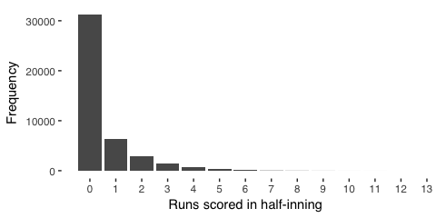
Building a bayesian run expectancy model
The model below uses the R package rstanarm’s interface to Stan’s fully-bayesian inferencing capabilities. We model RUNS_AFTER_EVENT as a function of (~) all combinations of RUNNERS and OUTS_CT, using neg_binomial_2 as we just discussed, and give our model the cleaned data rs. Absent including -1 in the formula, the model would use the first game state as a reference instead of separately reporting it with the other game states. It is not always appropriate to exclude this intercept, and we can google to learn more. The remaining options, QR = TRUE and chains = 1, iter = 500, cores = 4, seed = TRUE, have been described in depth here mc-stan.org/rstanarm/reference/stan_glm.html.
require(rstanarm)
fit <- stan_glm(RUNS_AFTER_EVENT ~ -1 + RUNNERS : OUTS_CT,
                family = neg_binomial_2,
                data = rs,
                QR = TRUE,
                chains = 1, iter = 500, cores = 4, seed = TRUE)
Model summary
We summarise the model,
summary(fit)##
## Model Info:
##
## function: stan_glm
## family: neg_binomial_2 [log]
## formula: RUNS_AFTER_EVENT ~ -1 + RUNNERS:OUTS_CT
## algorithm: sampling
## priors: see help('prior_summary')
## sample: 250 (posterior sample size)
## num obs: 184463
##
## Estimates:
## mean sd 2.5% 25% 50%
## RUNNERS0-0-0:OUTS_CT0 -0.7 0.0 -0.7 -0.7 -0.7
## RUNNERS1-0-0:OUTS_CT0 -0.1 0.0 -0.1 -0.1 -0.1
## RUNNERS0-2-0:OUTS_CT0 0.2 0.0 0.1 0.1 0.2
## RUNNERS0-0-3:OUTS_CT0 0.3 0.1 0.2 0.3 0.3
## RUNNERS1-2-0:OUTS_CT0 0.4 0.0 0.3 0.4 0.4
## RUNNERS1-0-3:OUTS_CT0 0.6 0.0 0.5 0.6 0.6
## RUNNERS0-2-3:OUTS_CT0 0.7 0.1 0.6 0.7 0.7
## RUNNERS1-2-3:OUTS_CT0 0.8 0.1 0.7 0.7 0.8
## RUNNERS0-0-0:OUTS_CT1 -1.3 0.0 -1.3 -1.3 -1.3
## RUNNERS1-0-0:OUTS_CT1 -0.7 0.0 -0.7 -0.7 -0.7
## RUNNERS0-2-0:OUTS_CT1 -0.4 0.0 -0.4 -0.4 -0.4
## RUNNERS0-0-3:OUTS_CT1 0.0 0.0 -0.1 -0.1 0.0
## RUNNERS1-2-0:OUTS_CT1 -0.1 0.0 -0.1 -0.1 -0.1
## RUNNERS1-0-3:OUTS_CT1 0.2 0.0 0.1 0.1 0.2
## RUNNERS0-2-3:OUTS_CT1 0.4 0.0 0.3 0.4 0.4
## RUNNERS1-2-3:OUTS_CT1 0.5 0.0 0.4 0.4 0.5
## RUNNERS0-0-0:OUTS_CT2 -2.2 0.0 -2.3 -2.3 -2.2
## RUNNERS1-0-0:OUTS_CT2 -1.5 0.0 -1.6 -1.5 -1.5
## RUNNERS0-2-0:OUTS_CT2 -1.1 0.0 -1.2 -1.2 -1.1
## RUNNERS0-0-3:OUTS_CT2 -1.0 0.0 -1.1 -1.1 -1.0
## RUNNERS1-2-0:OUTS_CT2 -0.8 0.0 -0.9 -0.9 -0.8
## RUNNERS1-0-3:OUTS_CT2 -0.8 0.0 -0.8 -0.8 -0.8
## RUNNERS0-2-3:OUTS_CT2 -0.6 0.1 -0.7 -0.7 -0.6
## RUNNERS1-2-3:OUTS_CT2 -0.3 0.0 -0.4 -0.3 -0.3
## reciprocal_dispersion 0.5 0.0 0.5 0.5 0.5
## mean_PPD 0.5 0.0 0.5 0.5 0.5
## log-posterior -158999.2 3.9 -159007.9 -159001.6 -158998.8
## 75% 97.5%
## RUNNERS0-0-0:OUTS_CT0 -0.7 -0.7
## RUNNERS1-0-0:OUTS_CT0 -0.1 -0.1
## RUNNERS0-2-0:OUTS_CT0 0.2 0.2
## RUNNERS0-0-3:OUTS_CT0 0.4 0.5
## RUNNERS1-2-0:OUTS_CT0 0.4 0.4
## RUNNERS1-0-3:OUTS_CT0 0.6 0.7
## RUNNERS0-2-3:OUTS_CT0 0.8 0.8
## RUNNERS1-2-3:OUTS_CT0 0.8 0.9
## RUNNERS0-0-0:OUTS_CT1 -1.3 -1.3
## RUNNERS1-0-0:OUTS_CT1 -0.7 -0.6
## RUNNERS0-2-0:OUTS_CT1 -0.3 -0.3
## RUNNERS0-0-3:OUTS_CT1 0.0 0.1
## RUNNERS1-2-0:OUTS_CT1 -0.1 0.0
## RUNNERS1-0-3:OUTS_CT1 0.2 0.3
## RUNNERS0-2-3:OUTS_CT1 0.4 0.5
## RUNNERS1-2-3:OUTS_CT1 0.5 0.5
## RUNNERS0-0-0:OUTS_CT2 -2.2 -2.2
## RUNNERS1-0-0:OUTS_CT2 -1.5 -1.5
## RUNNERS0-2-0:OUTS_CT2 -1.1 -1.1
## RUNNERS0-0-3:OUTS_CT2 -1.0 -1.0
## RUNNERS1-2-0:OUTS_CT2 -0.8 -0.8
## RUNNERS1-0-3:OUTS_CT2 -0.7 -0.7
## RUNNERS0-2-3:OUTS_CT2 -0.6 -0.5
## RUNNERS1-2-3:OUTS_CT2 -0.2 -0.2
## reciprocal_dispersion 0.5 0.5
## mean_PPD 0.5 0.5
## log-posterior -158996.6 -158993.0
##
## Diagnostics:
## mcse Rhat n_eff
## RUNNERS0-0-0:OUTS_CT0 0.0 1.0 250
## RUNNERS1-0-0:OUTS_CT0 0.0 1.0 250
## RUNNERS0-2-0:OUTS_CT0 0.0 1.0 250
## RUNNERS0-0-3:OUTS_CT0 0.0 1.0 250
## RUNNERS1-2-0:OUTS_CT0 0.0 1.0 250
## RUNNERS1-0-3:OUTS_CT0 0.0 1.0 250
## RUNNERS0-2-3:OUTS_CT0 0.0 1.0 250
## RUNNERS1-2-3:OUTS_CT0 0.0 1.0 250
## RUNNERS0-0-0:OUTS_CT1 0.0 1.0 250
## RUNNERS1-0-0:OUTS_CT1 0.0 1.0 250
## RUNNERS0-2-0:OUTS_CT1 0.0 1.0 250
## RUNNERS0-0-3:OUTS_CT1 0.0 1.0 250
## RUNNERS1-2-0:OUTS_CT1 0.0 1.0 250
## RUNNERS1-0-3:OUTS_CT1 0.0 1.0 250
## RUNNERS0-2-3:OUTS_CT1 0.0 1.0 250
## RUNNERS1-2-3:OUTS_CT1 0.0 1.0 250
## RUNNERS0-0-0:OUTS_CT2 0.0 1.0 250
## RUNNERS1-0-0:OUTS_CT2 0.0 1.0 250
## RUNNERS0-2-0:OUTS_CT2 0.0 1.0 250
## RUNNERS0-0-3:OUTS_CT2 0.0 1.0 250
## RUNNERS1-2-0:OUTS_CT2 0.0 1.0 250
## RUNNERS1-0-3:OUTS_CT2 0.0 1.0 250
## RUNNERS0-2-3:OUTS_CT2 0.0 1.0 250
## RUNNERS1-2-3:OUTS_CT2 0.0 1.0 250
## reciprocal_dispersion 0.0 1.1 32
## mean_PPD 0.0 1.0 250
## log-posterior 0.4 1.0 80
##
## For each parameter, mcse is Monte Carlo standard error, n_eff is a crude measure of effective sample size, and Rhat is the potential scale reduction factor on split chains (at convergence Rhat=1).Reviewing the model summary, n_eff and Rhats both look good. The various quantiles of coefficients are reported as the log of run expectancies because the model used neg_binomial_2 family, which defaults to a link function transforming these median estimates of our game states to log units. We can more easily interpret them by applying an exp(), as shown below along with organizing their median values into a matrix.
The median run expectancy matrix
The median run expectancy for each of the 24 game states are as follows,
# Extract and name coefficients from model
m <- exp(coef(fit))
m <- matrix(m, nrow = 8, ncol = 3, byrow = F)
rownames(m) <- levels(rs$RUNNERS)
colnames(m) <- levels(rs$OUTS_CT)

# Reorder rows according to bases
runners_on_base <-
  c("0-0-0", "1-0-0", "0-2-0", "0-0-3", "1-2-0", "1-0-3", "0-2-3", "1-2-3")
m <- m[match(runners_on_base, rownames(m)),]

# Show Matrix as Table
m
## 0 1 2
## 0-0-0 0.5110524 0.2682680 0.1068107
## 1-0-0 0.8927785 0.5117634 0.2193748
## 0-2-0 1.1664494 0.6953203 0.3179510
## 0-0-3 1.3992135 0.9726433 0.3545467
## 1-2-0 1.4842034 0.9216748 0.4308111
## 1-0-3 1.7917773 1.1931853 0.4676016
## 0-2-3 2.0476125 1.4653425 0.5341225
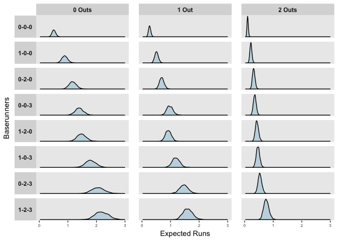
## 1-2-3 2.2020040 1.5968817 0.7635635More interestingly, we can also compare the distributions of expected runs for each game state,
# Extract posterior draws of the predictors, transform and reshape for plotting
pp <- as.data.frame(fit)
pp <- reshape2::melt(pp,
                     variable.name = "Game.State",
                     value.name="Expected.Runs")
pp <- transform(pp, Game.State = as.character(Game.State))
pp <- subset(pp, subset = Game.State != "reciprocal_dispersion")

# Separate Base States from Outs
pp <- transform(pp, Outs = substr(Game.State, start = 21, stop = 21))
pp <- transform(pp, Runners = substr(Game.State, start = 8, stop = 12))

# Reorganize order of Base States and Outs for a cleaner plot
pp <- transform(pp, Outs = factor(Outs,
                                  levels=c("0", "1", "2"),
                                  labels=c("0 Outs", "1 Out", "2 Outs")))
pp <- transform(pp,
      Runners = factor(Runners,
      levels=runners_on_base,
      labels=runners_on_base))

# Drop Unneeded Variables
pp$Game.State <- NULL

# Transform posterior estimates
pp <- transform(pp, Expected.Runs = exp(Expected.Runs))

# create the plot
ggplot(pp) +
  geom_density(aes(x = Expected.Runs), fill = "#C4D8E2") +
  facet_grid(Runners ~ Outs, scales = "free_y", switch = "y") +
  theme_gray() +
  theme(axis.text.x = element_text(size = 6),
        axis.text.y = element_blank(),
        axis.ticks.y = element_blank(),
        strip.text.x = element_text(size = 9, face = "bold"),
        strip.text.y = element_text(size = 9, face = "bold", angle = 180),
        panel.grid.minor = element_blank(),
        panel.grid.major = element_blank(),
        panel.spacing.x = unit(1, "lines")) +
  labs(x = "Expected Runs", y = "Baserunners")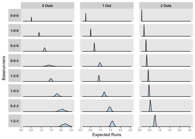
The distributions above reflect the model’s uncertainty in the predictors, but importantly, when predicting or forecasting, we need to consider both this uncertainty and the natural variation in events. The mean posterior estimates of observed at bats in the 2017 season are shown below.
# combine preditions with original data
yrep <- posterior_predict(fit)
rs <- cbind(rs, yrep = colMeans(yrep))

# reorder levels for RUNNERS and OUTS_CT
# Reorganize order of Base States and Outs for a cleaner plot
rs <- transform(rs, Outs = factor(as.character(OUTS_CT),
                                  levels=c("0", "1", "2"),
                                  labels=c("0 Outs", "1 Out", "2 Outs")))
rs <- transform(rs,
      Runners = factor(as.character(RUNNERS),
      levels=runners_on_base,
      labels=runners_on_base))

# plot posterior estimates from original data
ggplot(rs) +
  geom_density(aes(x = yrep), fill = "#C4D8E2") +
  facet_grid(Runners ~ Outs, scales = "free_y", switch = "y") +
  theme_gray() +
  theme(axis.text.x = element_text(size = 6),
        axis.text.y = element_blank(),
        axis.ticks.y = element_blank(),
        strip.text.x = element_text(size = 9, face = "bold"),
        strip.text.y = element_text(size = 9, face = "bold", angle = 180),
        panel.grid.minor = element_blank(),
        panel.grid.major = element_blank(),
        panel.spacing.x = unit(1, "lines")) +
  labs(x = "Expected Runs", y = "Baserunners")