In R’s grammar of graphics package (ggplot2), we can encode data in custom-made glyph shapes from vector graphics and encode its size, fill color, or both. SVG graphics display lines, colors fills using paths. Let’s make an SVG graphic containing a single path of a complex shape, assign the graphic in R to data, and change its attributes. For this exercise, I’ve created an SVG path of the silhouette of a baseball player (using Inkscape)¹. Here are the resulting coordinates of its SVG path², which I saved as a string into an R object:

path <- "380.5,141 382.3,142 397.6,148.6 402.5,158.5 403.5,163.6 403.5,168.7 407.3,171.6 408.4,182.9 404.5,188.3 404.5,194.7 404.5,200.5 409,200 413.3,201.8 415.9,213.6 423.5,220.9 426.9,224.8 433.8,240.9 435.4,249.2 435.5,259.7 436.7,273.7 437.7,280.8 438.5,288.4 438.5,295.9 438.6,314.4 437.3,333.5 434.7,345.3 434.4,349.1 440.4,364.6 438,367 430.8,367 429.6,373.5 430.4,384.6 420.2,409.9 403.2,424.1 398.6,428.9 396,432.9 390.5,438.6 385.6,446.6 381.6,458.9 374.2,476.8 369.6,486.4 366.6,496.7 366.5,505.4 370.4,511.6 373.5,523.7 376.5,535 377.5,539.6 378.5,543.7 378.5,545.1 379.5,579.7 379.6,598.7 382.6,615.9 385.2,619.2 387.3,635.2 384.3,650.6 378.1,652 371.1,652 364.9,651.2 358.9,650.1 356.5,650 343.5,650.1 332.5,652.5 332.5,653 329.5,653 329.5,651.2 323.7,650.2 317.7,650.8 315.1,646.8 306.9,647.6 304.6,643.2 304.6,636.5 308.4,633.1 313.9,632 320,631 321,631 341.4,623.6 351.6,614.3 354.5,609.3 354.3,597.1 352.6,584.9 349.2,573.3 343,556.9 340.6,548.9 337.5,536.6 335.7,530.9 330.1,519.2 323.8,506.8 323.5,504.4 323.5,489.9 324.5,483.3 325.3,477.2 324.7,469.6 324.5,467.2 327.7,449.5 330.3,440.6 332.7,432 335.5,421.2 338.4,410.4 340.6,398.8 341.6,384.8 314.5,356.4 299.5,337.6 295,332 293.5,340.4 291.4,348.5 280.1,367.8 268.2,386 265.4,393.3 258.5,411.8 258.5,417.4 256.3,426.5 244.4,447.6 241.8,450.4 237.5,447.5 229.4,444 223.4,438.8 219.1,434.1 207.6,425.6 204.5,424.6 193.5,421.5 183.2,413.9 175.7,407.5 174.5,401.5 175.5,395.5 178.8,392.2 191.2,394.2 195.9,396 201.2,397.9 206.2,399 222.8,399.9 240.7,387.6 249.5,364.3 252.6,348.1 257.8,330.2 260.5,319.3 261.5,313.7 262.3,308.1 261.5,302.1 269.3,292 269.3,288.7 271.2,286.7 277.9,281.3 285.4,280 309.2,285.3 322.1,290.5 317.3,282.2 311.9,275.1 310,274.9 306.4,268.8 306.2,261.5 305.4,250.6 302.7,243.2 300.1,239.1 296.1,239.1 289.5,232.5 284.4,226.4 281.5,229.4 281,228.7 268,231.1 269.7,229.2 262.5,228.8 273.5,226.9 283.3,221.4 285.3,210.1 286.6,202.1 290.5,189.7 293.5,186 299.9,178.1 304.5,176 321.2,170 334.4,174 339.6,175.8 343.4,180.6 346.5,189.9 346.5,191.3 346.7,202.4 347.3,210.5 342,224.8 340.5,229.7 339.6,243.4 343.2,239.7 351.6,236 368.7,226.7 367.2,221.3 364.6,210.9 361.3,199.2 360,195.9 353.9,188.8 352.2,178.4 354.5,174.2 353.5,163.6 357.8,150.4 368.8,142.1 372.5,141 380.5,141"

Next, we convert the SVG path string to a data.frame. The path above is read as a series of x,y coordinates, each time followed by a space. See MDN contributors, Paths. In moz://a, MDN Web Docs. Last Updated 2020 April 5.. We can accomplish this in many ways. Let’s use a few string manipulation functions from base R: gsub to replace spaces with commas:

path <-  gsub(' ', ',', path)

then split the string using the commas using strsplit:

path <-  as.numeric(unlist(strsplit(path, ',')))

leaving odd elements as x-coordinates, and even elements as y-coordinates. Organize these into a data.frame like so:

glyph <- data.frame(xsh = path[ c(T,F) ],
                    ysh = path[ c(F,T) ],
                    id  = 1)

Of note, I give an id to this glyph, which is the same for each point within. Finally, I made the glyph coordinates, as mentioned, in Inkscape, where the origin of its coordinate system, (0,0) starts in the upper, left corner and the y-values increase going down. We will center our glyph and flip it by subtracting each coordinate by the mean of each coordinate. We will also scale the values so the maximum dimension is 1 unit:

glyph$xsh <- with(glyph, (mean(xsh) - xsh) / dist( range(xsh, ysh) ) )
glyph$ysh <- with(glyph, (mean(ysh) - ysh) / dist( range(xsh, ysh) ) )

Using ggplot, our glyph looks like:

library(ggplot2)

ggplot(glyph) + 
  theme_minimal() +
  coord_equal() +
  geom_polygon(aes(x = xsh, 
                   y = ysh, 
                   group = id),
               color = 'black', 
               fill = 'lightblue') +
  labs(x = 'x coordinates', 
       y = 'y coordinates')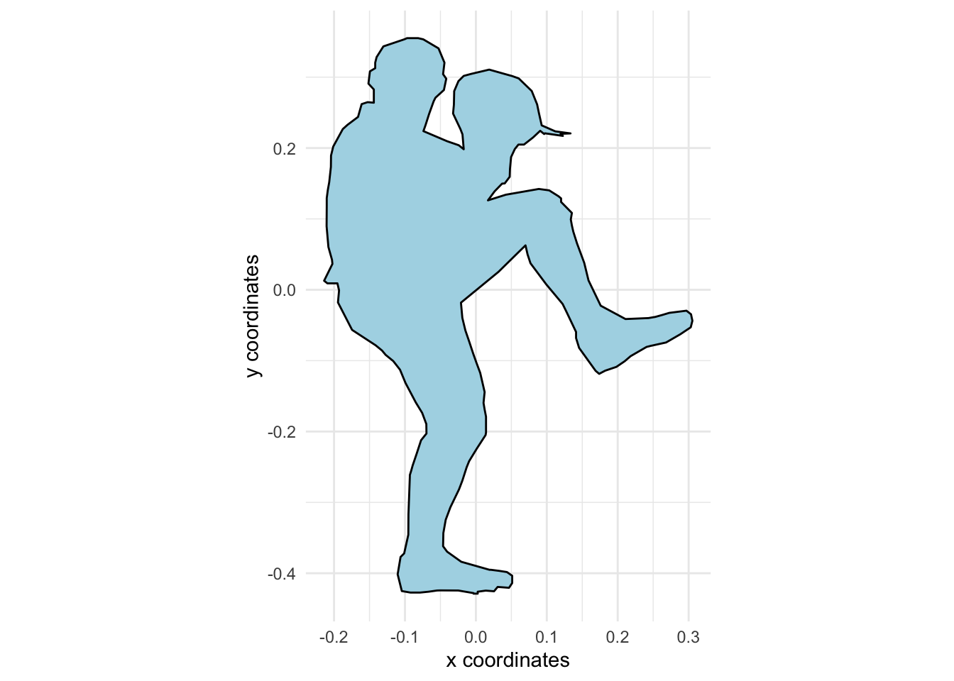

Great, we now have a glyph we can encode place, size, and color according to our data. To illustrate this, let’s create a few random numbers for x, y, and size values that we’ll use as our observed data:

d <- data.frame(x = rnorm(10, 50, 5),
                y = rnorm(10, 30, 5),
                size = rnorm(10, 4, 1))

We need to add a couple more variables to the data frame: data observation number and glyph id, which we use to merge the glyph dataframe into the observed data:

d$observation <- seq_len( NROW(d) )
d$id <- 1
d <- merge(d, glyph)

To place and size the glyphs, we multiply the glyph coordinates (xsh, ysh) by our size values (size) and add the data coordinates (x, y):

ggplot(d) + 
  theme_minimal() +
  theme(legend.position = '') +
  coord_equal() +
  geom_polygon(aes(x = x + xsh * size, 
                   y = y + ysh * size, 
                   group = observation,
                   fill = size), 
               color = "black") +
  labs(x = 'x coordinates', 
       y = 'y coordinates')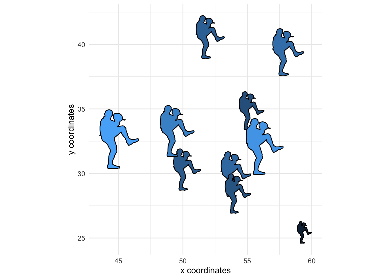

It is now easy to see other ways to encode the glyph, like rotating it based on data values, or combining multiple glyph components, each with its own value and grouping them as, for example, shown in publications, Creating and placing custom glyphs.