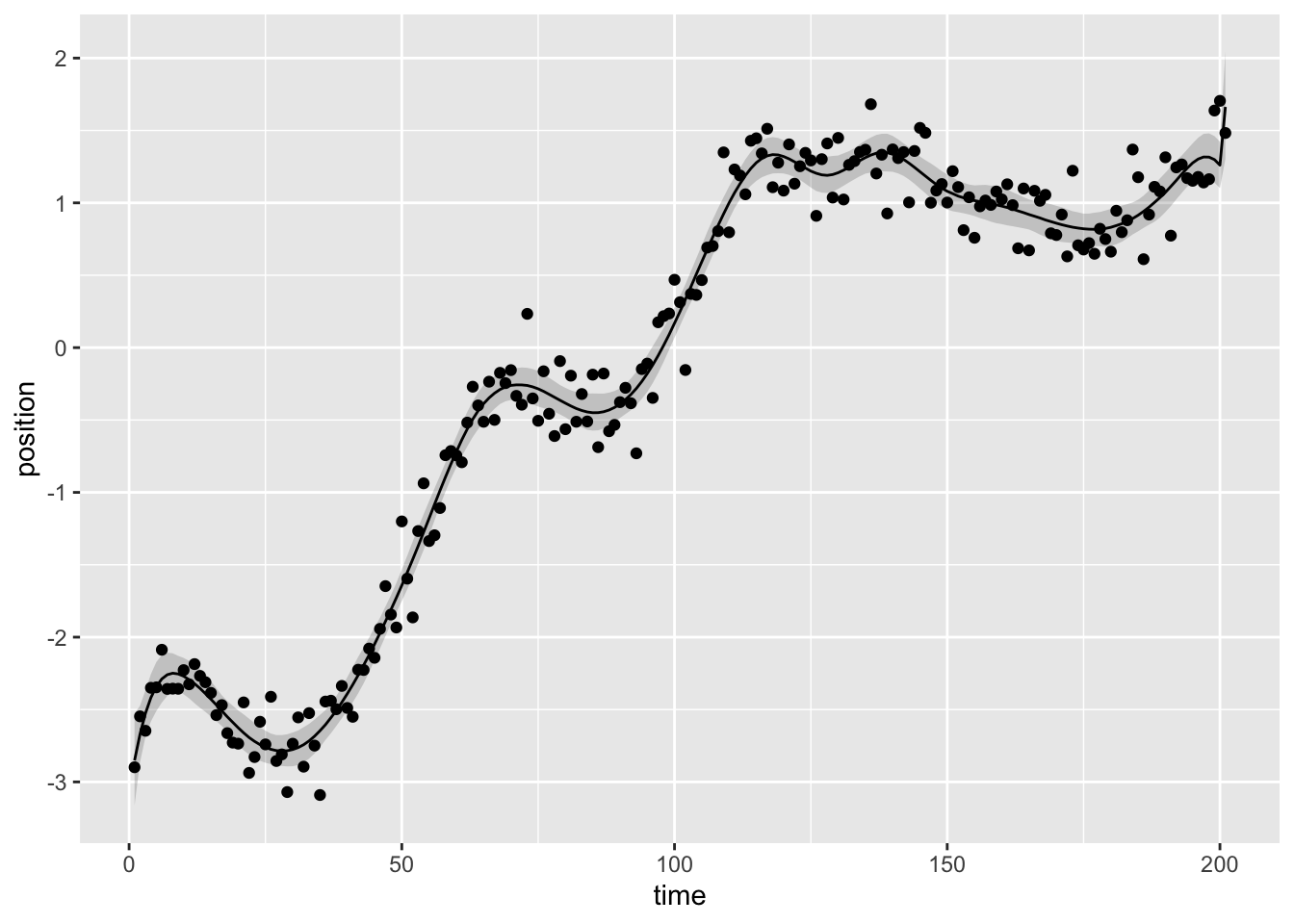
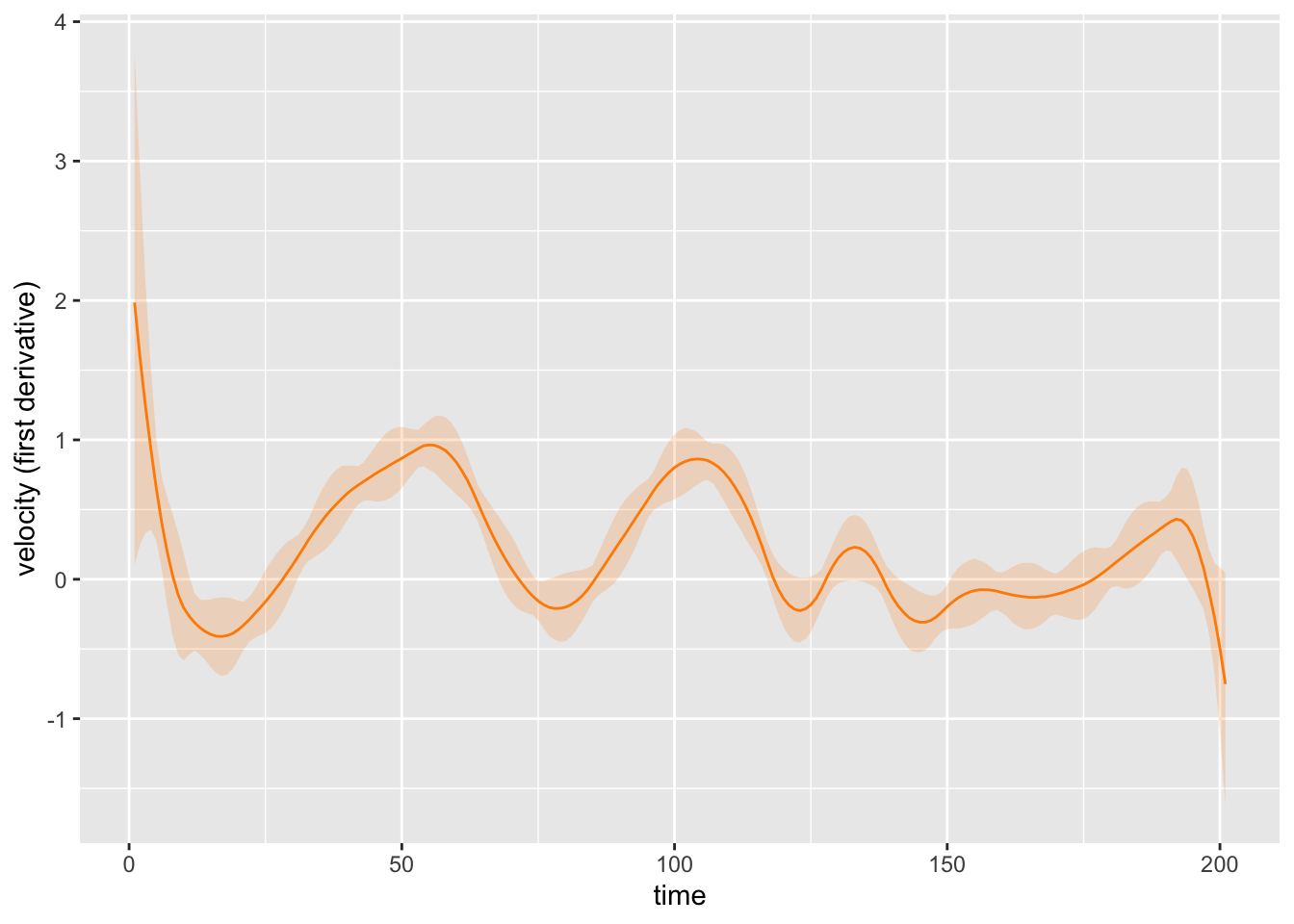
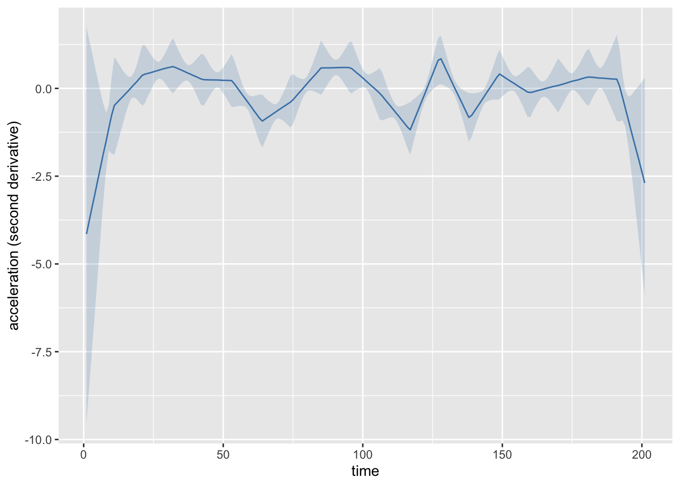
In the last post, I showed how we can speed up computation for splines in Stan. This post is, ahem, derivative. Perhaps we have noisy data of position and time, and we want to estimate speed and acceleration. We can use b-splines and their derivatives for this.

So let’s pick up where we left off, and add calculations in Stan to calculate the first and second derivatives of the spline in Stan. Much of the code below mirrors that of the previous post. There are multiple approaches to calculating derivatives of splines. We can take the derivative of the basis functions (Rogers 2001, sec. 3.10 B-Spline Curve Derivatives) or we can difference the coefficients (Boor 2001, X. The Stable Evaluation of B-Splines and Splines). In the Stan functions block below, I’ve added calculations for the first and second derivatives of the basis functions.

functions {
  
  tuple(vector, vector, vector) build_b_spline(vector x, array[] real ext_knots, 
                        int ind, int k) {
    
    int n_x = size(x);
    vector[n_x] zeros = rep_vector(0, n_x);
    // basis functions & weights
    vector[n_x] d0, w1 = zeros, w2 = zeros;
    // first derivative & weights
    vector[n_x] d1, f1 = zeros, f2 = zeros, f3 = zeros, f4 = zeros;
    // second derivative & weights
    vector[n_x] d2, s1 = zeros, s2 = zeros, s3 = zeros, s4 = zeros;
    
    if (k == 1) {
      
      // first order splines
      for (i in 1:n_x) {
        d0[i] = (ext_knots[ind] <= x[i]) && (x[i] < ext_knots[ind + 1]); 
        d1[i] = 0;
        d2[i] = 0;
      }
        
    } else {
    
      // calculate weights for b, b', b"
      if (ext_knots[ind] != ext_knots[ind + k - 1]) {
        w1 = (x - rep_vector(ext_knots[ind], n_x))   
           / (ext_knots[ind + k - 1] - ext_knots[ind]);
        f1 = rep_vector(1, n_x) 
           / (ext_knots[ind + k - 1] - ext_knots[ind]);
        f3 = w1;
        s1 = rep_vector(2, n_x) 
           / (ext_knots[ind + k - 1] - ext_knots[ind]);
        s3 = w1;
      }
      
      if (ext_knots[ind + 1] != ext_knots[ind + k]) {
        w2 = 1 - (x - rep_vector(ext_knots[ind + 1], n_x)) 
           / (ext_knots[ind + k] - ext_knots[ind + 1]);
        f2 = rep_vector(-1, n_x) 
           / (ext_knots[ind + k] - ext_knots[ind + 1]);
        f4 = w2;
        s2 = rep_vector(-2, n_x) 
           / (ext_knots[ind + k] - ext_knots[ind + 1]);
        s4 = w2;
      }

      // calculate b, b', b"
      tuple(vector[n_x], vector[n_x], vector[n_x]) b1 = 
        build_b_spline(x, ext_knots, ind, k - 1);
      tuple(vector[n_x], vector[n_x], vector[n_x]) b2 = 
        build_b_spline(x, ext_knots, ind + 1, k - 1);
      
      d0 = w1 .* b1.1 + w2 .* b2.1;
      d1 = f1 .* b1.1 + f2 .* b2.1 + f3 .* b1.2 + f4 .* b2.2;
      d2 = s1 .* b1.2 + s2 .* b2.2 + s3 .* b1.3 + s4 .* b2.3;
    }

    return( (d0, d1, d2) );
  
  }
  

  tuple(matrix, matrix, matrix) build_B(int degree, int T, array[] real t, 
                 int X, vector x) {
    
    tuple(matrix[T + degree - 1, X],
          matrix[T + degree - 1, X],
          matrix[T + degree - 1, X]) B;
    
    tuple(vector[X], vector[X], vector[X]) bv;
    
    array[2 * degree + T] real ext_knots =
    append_array(append_array(rep_array(t[1], degree), t), rep_array(t[T], degree));
    for (ind in 1:(T + degree - 1)) {
      bv = build_b_spline(x, ext_knots, ind, degree + 1);
      B.1[ind,:] = to_row_vector(bv.1);
      B.2[ind,:] = to_row_vector(bv.2);
      B.3[ind,:] = to_row_vector(bv.3);
    }
      
    B.1[T + degree - 1, X] = 1;
  
    return B;
  }
  
  
}


data {
  
  int<lower=1> X;                 // number of times measured
  vector[X] x;                    // each time point measured
  vector[X] y;                    // the measurement at each time point x
  
  int<lower=1> T;                 // number of knots
  array[2] real xb;               // boundary knot locations (outside data)
  int<lower=1> degree;            // degree of the spline
  int<lower=0,upper=1> penalized; // whether to use prior for smoothing
  
}


transformed data {
  
  // T number of knots t created at evenly-spaced quantiles of data x
  array[T] real p;
  for(i in 1:T) p[i] = (i - 1.0) / (T-1.0);
  array[T] real t = quantile(append_row(xb[1], append_row(x, xb[2])), p);

  // build the spline matrix B, B', and B" and decompose B
  int n_basis = T + degree - 1; 
  
  tuple(matrix[n_basis, X],
        matrix[n_basis, X],
        matrix[n_basis, X]) B = build_B(degree, T, t, X, x);
  
  matrix[X, n_basis] Q_ast = qr_thin_Q(B.1') * sqrt(X - 1);
  matrix[n_basis, n_basis] R_ast = qr_thin_R(B.1') / sqrt(X - 1);
  matrix[n_basis, n_basis] R_ast_inverse = inverse(R_ast);
  
  // helpers
  vector[X] zeros_X = rep_vector(0, X);
}


parameters {
  
  vector[n_basis] theta_raw; // coefficients on Q_ast
  real<lower=0> sigma;       // scale of the variation
  real<lower=0> tau;         // penalization on wiggles
  
}


transformed parameters {
  
  // coefficients for Q_ast, orthogonal 
  // projection of basis function B
  vector[n_basis] alpha;
  
  // random walk to smooth "wigglyness"
  if(penalized) {
    alpha[1] = theta_raw[1];
    for(i in 2:n_basis) alpha[i] = alpha[i-1] + theta_raw[i] * tau;
  } else {
    alpha = theta_raw * tau;
  }

}


model {
  
  theta_raw ~ normal(0, 1);
  tau ~ normal(0, 1);
  sigma ~ exponential(1);  
  y ~ normal_id_glm(Q_ast, zeros_X, alpha, sigma);

}


generated quantities {
  
  vector[n_basis] beta = R_ast_inverse * alpha;
  vector[X] y_hat = B.1' * beta;
  vector[X] dydt1 = B.2' * beta;
  vector[X] dydt2 = B.3' * beta;
  
}

To calculate the derivative basis functions, we simply pass in which derivative we want to the main function build_B, where deriv \(\in \{0,1,2\}\) for none, first, and second derivative, respectively.

To demonstrate, the program above calculates all three, the basis function, the first derivative, and the second derivative in the transformed data block.

Then, to estimate those derivatives, we matrix multiply those with our coefficients, here beta, which I’ve calculated in generated quantities.

Let’s see how the first and second derivative estimates play out from the simulated data of the last post: