Deriving velocity and position as a function of time

In that context, we begin with Newton’s second law of motion: \(F = ma\) where acceleration \(a\) is the derivative of velocity. Thus, the net force of that the runner produces \(F_{\text{net}} = m \dot{v}(t)\). Net force consists of both propulsive and resistive forces: \(F_{\text{net}} = F_{\text{propulsive}} + F_{\text{resistive}}\).

Propulsive force \(F_{\text{propulsive}}\) depends on the runner’s fitness and effort that is less than or equal to his maximum effort.

Resistive forces \(F_{\text{resistive}}\) depend on, for example, runner size, biological inefficiencies, and air resistance. Keller (1973) defines this force as proportional to the runner’s mass and velocity to excellent results: \(F_{\text{resistive}} = -k m v(t)\) where \(k \ge 0\).

All together, we have the ordinary differential equation,

\[ m \dot{v}(t) = m F_{\text{propulsive}} - kmv(t) \] As runner mass \(m\) cancels out, this simplifies,

\[ \dot{v}(t) = F_{\text{propulsive}} - kv(t) \]

For times when we can assume an initial condition \(v(0) = 0\), we can solve the system of ordinary differential equations by solving the separable equation,

\[ \frac{dv(t)}{dt} = F_{\text{propulsive}} - kv(t) \] such that \(v(0) = 0\). We divide both sides by \(F_{\text{propulsive}} - kv(t)\):

\[ \frac{\frac{dv(t)}{dt}}{F_{\text{propulsive}} - kv(t)} = 1 \]

and integrate both sides with respect to \(t\):

\[ \int \frac{\frac{dv(t)}{dt}}{F_{\text{propulsive}} - kv(t)}dt = \int 1 dt \]

Then evaluate the integrals. For the integral,

\[ \int \frac{1}{F_{\text{propulsive}} - kt} \] substitute \(u = F_{\text{propulsive}} - kt\) and \(du = -kdt\):

\[ =-\frac{1}{k} \int \frac{1}{u}du \] The integral of \(1/u\) is \(\text{log}(u)\) plus a constant:

\[ = - \frac{\text{log}(u)}{k} + c \]

substituting back for \(u = F_{\text{propulsive}} - kt\), we get:

\[ = - \frac{\text{log}(F_{\text{propulsive}} - kt)}{k} + c \]

The right side integral of \(1\),

\[ \int 1 dt \]

is simply: \(=t + c\).

Next, we solve for \(v(t)\):

\[ - \frac{\text{log}(F_{\text{propulsive}} - kv(t) )}{k} = t + c \] Multiplying both sides by \(-k\), we get:

\[ \text{log}(F_{\text{propulsive}} - kv(t))= -kt -kc \] and cancel the logarithm:

\[ F_{\text{propulsive}} - kv(t) = e^{-kt - kc} \] Subtracting \(F_{\text{propulsive}}\) from both sides and dividing by \(-k\):

\[ v(t) = \frac{F_{\text{propulsive}}}{k} - \frac{e^{-kt - kc}}{k} \]

We solve for \(c\) using initial conditions, substituting \(v(0)=0\) into the above equation:

\[ \frac{-e^{-kc}+F_{\text{propulsive}}}{k}=0 \] Rearranging, we get \(c\):

\[ c = - \frac{\text{log}(F_{\text{propulsive}})}{k} \]

Substituting \(c\):

\[ v(t) = \frac{F_{\text{propulsive}} - F_{\text{propulsive}} e^{-kt}}{k} \]

Now that we have analytically derived velocity as a function of time, we can substitute it back into our first principles based ODE with parameters for runner’s propulsive force and resistive parameters where we’ll also substitute \(t - t_0\) for \(t\) to account for delay or reaction time in beginning the run,

\[ \begin{equation} x(t) = \frac{F_{\text{propulsive}_p}}{k_p} \cdot (e^{-k_p (t - t_0)} - 1 + k_p \cdot (t - t_0)) \tag{1} \end{equation} \]

we can estimate \(\textbf{F}_\text{propulsive}\) and \(\textbf{k}\) in Stan. Once estimated, we can calculate maximum velocity,

\[ \begin{equation} v_\text{max} = F_\text{propulsive} / k \tag{2} \end{equation} \]

as well as calculate position and velocity given time (e.g., time from bat-ball contact to intercept with ground), or the other way around: we may calculate time given distance traveled:

\[ t(x) = \frac{1 + (k^2 x)/F + W(-e^{-1 - (k^2 x)/F)})}{k} + t_0 \]

where \(W(\cdot)\) is the Lambert W function.

This would help us estimate the probability that a fielder catches a fly ball given his location, the ball’s landing location and speed; the probability of stealing a base given the runner’s lead-off, pitch speed and catcher pop time; and many other questions. After all, scoring runs and — ultimately — wins always depend on running speed except for strikeouts and home runs.

Estimating runner propulsive and resistive forces

Bayesian inference is a preferred method of estimating unknown parameters in a way that fully expresses variation in those parameters. In the below model, we use time-stamped distances for a runner, estimate runner-specific parameters for propulsive force \(P\) and their running inefficiencies \(k\), the latter of which is partially-pooled towards a population (they share biology and air resistance, for example), and estimate the variation in our estimates from the observations.

Stated mathematically, the model estimates \(\textbf{F}_\text{propulsive}\) and \(\textbf{k}\) from equation (1) as follows:

\[ \begin{align} x_{p[t]} &\sim N(\mu_{p[t]}, \sigma) \\ \mu_{p[t]} &= \frac{F_{\text{propulsive}_p}}{k_p} \cdot (e^{-k_p (t - t_0)} - 1 + k_p \cdot (t - t_0)) \\ \sigma &\sim \text{normal}^+(0,1) \\ \textbf{F}_\text{propulsive} &\sim \text{exponential}(0.1) \\ \textbf{k} &\sim \text{normal}(\mu_k, \sigma_k) \\ \mu_k &\sim \text{exponential}(1) \\ \sigma_k &\sim \text{normal}^+(0,1) \\ \end{align} \]

Finally, we estimate maximum velocities from the model to compare against published estimates. Let’s put this model to work.

Example inferences: Statcast sprint speed leaderboard

Baseball Savant maintains a “sprint speed” leaderboard, from seasons 2015 through the present. These summarize game data in a couple of ways. First, they define “sprint speed” as,

Sprint Speed is Statcast’s foot speed metric, defined as “feet per second in a player’s fastest one-second window” on individual plays. For a player’s seasonal average, the following two types of plays currently qualify for inclusion in Sprint Speed. The best of these runs, approximately two-thirds, are averaged for a player’s seasonal average.

• Runs of two bases or more on non-homers, excluding being a runner on second base when an extra base hit happens
• Home to first on “topped” or “weakly hit” balls.

The Major League average on a “competitive” play is 27 ft/sec, and the competitive range is roughly from 23 ft/sec (poor) to 30 ft/sec (elite). A Bolt is any run above 30ft/sec. A player must have at least 10 competitive runs to qualify for this leaderboard. Read more about how Sprint Speed works here.

Their calculations do not really represent a player’s ability to run. For example, biologically, players decline in underlying sprint speed starting around age 30 (Moore 1975) but the sprint speed leaderboard shows 60 percent of players having a higher year-over-year sprint speed after age 30. Further, their method uses observational data wherein each player has differing numbers of runs that Statcast has identified as “competitive”, differing player intentions on those runs, and over varying distances. Top speed in a sprint requires between 60-80 meters of full effort (just over a double), but the arbitrary subset of runs that Statcast averages includes singles, among other things.

We’ll test for bias in the leaderboard using a second form of data provided. Along with “sprint speed,” the website provides “90ft running splits”, which include an imperfect summary of a player’s best times from home plate to first base at every five feet.

We’ll use these times to estimate the players’ force and inefficiencies, and then compare those to the estimates of sprint speed.

Our physics-based model recovered estimates of position within a standard deviation of 0.49 foot from the observed splits every five foot.

Using those same estimates, we can calculate an estimated maximum velocity (equation (2)) and compare those to Savant’s sprint speed leaderboard. Doing so,

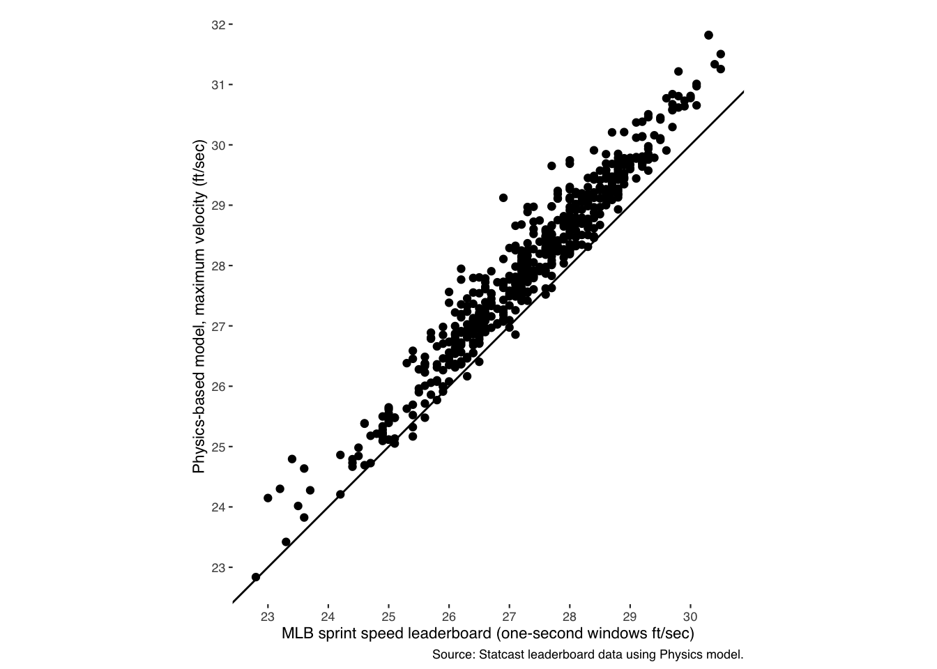
Figure 1: Modeling max running speed from 90-ft running splits reveals systematic bias in sprint speed leaderboard.

we learn from modelling the additional information from Savant’s splits that their method for calculating sprint speed systematically underestimates player ability, even using Statcast’s same method for collecting the data.

Aside from more accurately estimating maximum velocity of runners, this approach adds the ability to estimate position or speed at any point along a run¹, around the bases or in the field.

Hopefully, this post helps demonstrate the power of including dynamic structures governed by physics in a Bayesian framework, and the insights that it can bring.