Let’s practice expressing a probabilistic model aided by physics. Physics have been used, of course, to mathematically describe the forces involved in running short distances. To estimate sprint speed we can inform our models with basic anatomical information and physics. The mathematical physics of running speed depend on body weight, and stride length and rate. Let’s begin with those.

Let’s start with physics equations to describe speed, and accelerating to maximum speed. We can express this by considering acceleration per stride, as explained in Herman (2016). Imagine stepping into the starting blocks on a 100m sprint. On the first push with our legs, we accelerate to a speed \(v_1\) at the end of the stride from a force \(F\) moved by a distance \(L\). To accelerate, we must produce the required work \(W\), as force \(F\) times stride length \(L\) — all together, \(W = FL\) — further expressed by the kinetic energy in our body, \(\frac{1}{2}ma\), or more specifically, \(\frac{1}{2}(m_{\text{b}} - 2m_{\text{leg}})v_1^2\), with one leg in the air \(\frac{1}{2}m_{\text{leg}}v_1^2\). After the first stride, then, we can express our speed or velocity as,

\[ v_1^2 = \frac{2FL}{m_{\text{b}}- m_{\text{leg}}} \]

In the next stride, we’ve switched feet doing the work, again \(FL\), but accelerate the body from \(v_1\) to \(v_2\) and the first leg from \(0\) to \(v_2\), thus,

\[ v_2^2 = \frac{2FL}{m_{\text{b}} - m_{\text{leg}}} \left( 1 + \frac{m_{\text{b}} - 2m_{\text{leg}}}{m_{\text{b}} - m_{\text{leg}}} \right) \]

For \(n\) strides,

\[ v_n^2 = \frac{2FL}{m_{\text{b}} - m_{\text{leg}}} \left( 1 + \frac{m_{\text{b}} - 2m_{\text{leg}}}{m_{\text{b}} - m_{\text{leg}}} + \left( \frac{m_{\text{b}} - 2m_{\text{leg}}}{m_{\text{b}} - m_{\text{leg}}} \right)^2 +\dots+\left( \frac{m_{\text{b}} - 2m_{\text{leg}}}{m_{\text{b}} - m_{\text{leg}}} \right)^n\right) \]

Notice that these accelerations follow the pattern of a geometric series \(1 + x + x^2 + \dots + x^n = (1 - x^n) / (1 - x)\) for \(0 < x < 1\). Thus, the series approaches a final running velocity of,

\[ v_{n \rightarrow \infty}= \sqrt \frac{2FL}{m_{\text{leg}}} \]

Empirical studies provide an expected leg mass \(m_{\text{leg}}\) around \(0.161m_{\text{b}}\) see Herman (2016). As with leg mass, empirical studies have estimated stride length as a function of human height, though stride length will also depend on run technique and generated forces. Those experiments measured stride lengths during short distances between around 1.14 to 1.35 times runner height in meters, see Rompottie (1972) and Hoffman (1972). To estimate a new run speed, we can estimate our force, given observations of previous sprints through modeling.

Let’s code the beginning of a simplified model that reflects these measures and assumptions using Stan, a probabilistic programming language. Take some time to compare the mathematical description above with the code below:

data {

// runner and event information

  int<lower=0> N;          // count runs
  array[N] int<lower=0> r; // runner index
  vector<lower=0>[N] t;    // time s
  vector<lower=0>[N] d;    // distance m
  vector<lower=0>[N] m;    // body mass kg
  vector<lower=0>[N] h;    // body height m

}

transformed data {
  int n_r = max(r);                     // count unique runners
  vector<lower=0>[N] L = 1.35 * h;      // stride length, m
  vector<lower=0>[N] m_leg = 0.161 * m; // lifted leg weight, kg
}

parameters {
  vector<lower=0>[n_r] F; // force each runner, Newtons (kg m / s^2)
  real<lower=0> F_pop;    // force population, Newtons (kg m / s^2)
  real<lower=0> sigma;    // overall variation, m / s
}

model {

  // priors
  F_pop ~ normal(250, 20);
  F ~ normal(F_pop, 50);
  sigma ~ exponential(5);

  // likelihood  
  vector[N] mu = sqrt(2 * F[r] .* L ./ m_leg);
  target += normal_lpdf( d ./ t | mu, sigma);
}

generated quantities {
  array[N] real 
    t_hat = normal_rng(sqrt(2 * F[r] .* L ./ m_leg), sigma);
}

Let’s fit this simplistic model to, say, winning Olympic male sprinters. We can pull their race information from Wikipedia, along with each winner’s height and weight from their biographies with the caveat that those anthropometric values are general and do not necessarily reflect their height and weight at the time of their winning race. Thus, this model fit is merely illustrative. Here are the data:

Let’s fit the model with these data.

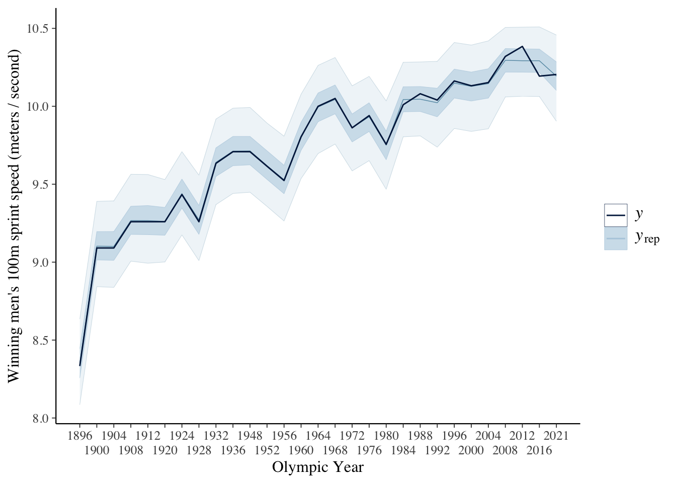
Running a posterior predictive check, we find that our estimates include the data:

Here are our estimates of the forces each winner produced:

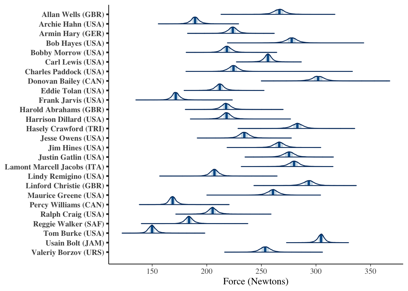
Now, in this simplified example, I included prior experimental values for leg mass \(m_{\text{leg}}\) and stride length \(L\), but these are not precise for our particular sprinters. We can propagate variation and uncertainty in these by estimating them as random variables, informed by past observations. Further, the prior information assigned was illustrative, and not informative. With more care in those priors, we can more accurately model these forces. Of note, we estimated each winner’s forces as separate parameters, informed by a hyper-prior of the average forces generated by the population.

What can we use these parameters for? Well, we might draw from a particular winner’s estimates to see what a new race may have resulted in. Or we may use the population information to estimate what a new winning sprinter may have generated. But, certainly, there are limitations in the use of this model as is. If we were to extend the model, better uses might be to try to include models for, say, maximum expected forces possible in tomorrow’s Olympic races. To get started, consider some ideas in Noubary (2010). Or we may consider including models of change in runner forces as they age.

Stay curious.