Estimating human limits of running speed
Prefontaine “finally got it through my head that the real purpose of running isn’t to win a race. It’s to test the limits of the human heart. And that he did. Nobody did it more often. Nobody did it better.”
— Bill Bowerman.
We’ve been recording progress towards those limits, whatever they are, for some time. World records have been collected for running distances, from 50 meters on an indoor track to marathons and beyond. These records also include single-age records. Just what may be the limits that “Pre” pushed to test in running, and how might those limits depend on our age?
Fair and Kaplan (2018) explored these questions across some ages and some distances. In this post, I aims to explore and extend their analysis using Bayesian methods of estimation.
Available records
A world, governing body for running events — World Athletics — maintains records for various distances. To be a reliable and comparable record, the run must comply with certain conditions. Those records include, among other things, the event distance and run date, competitor’s name, date of birth, nationality, the marked time, and a world ranking. These events include short and lond distance, and indoor and outdoor.
Along with these data, single-age world records are maintained for longer distance events, from 3,000 meters to marathon, by The Association of Road Racing Statisticians (ARRS). ARRS is an independent, non-profit organization that collects, analyses, and publishes results and statistics regarding elite distance running at distances 3000m and longer. Here are the observed measures:
Variable | Type | Min | Distribution | Max | Distinct |
nationality | String/Factor | ALG |
| WAL | 57 |
run_loc_city | String/Factor | Aachen |
| Zurich | 731 |
run_loc_country | String/Factor | ALG |
| WAL | 64 |
runner | String/Factor | Aaron West... |
| Zoya Ivano... | 936 |
runtime | String/Factor | 00:10:02.3... |
| 9:53:48 | 2184 |
sex | String/Factor | female |
| male | 2 |
type | String/Factor | indoor tra... |
| road | 3 |
units | String/Factor | Kilometers |
| Miles | 2 |
birthdate | Date | 1895-01-19 |
| 2013-06-20 | 923 |
rundate | Date | 1965-05-30 |
| 2020-02-16 | 1510 |
age | Numeric | 3.92 |
| 98.36 | 2248 |
distance | Numeric | 3 |
| 30 | 11 |
runtime_sec | Numeric | 440.67 |
| 35628 | 2175 |


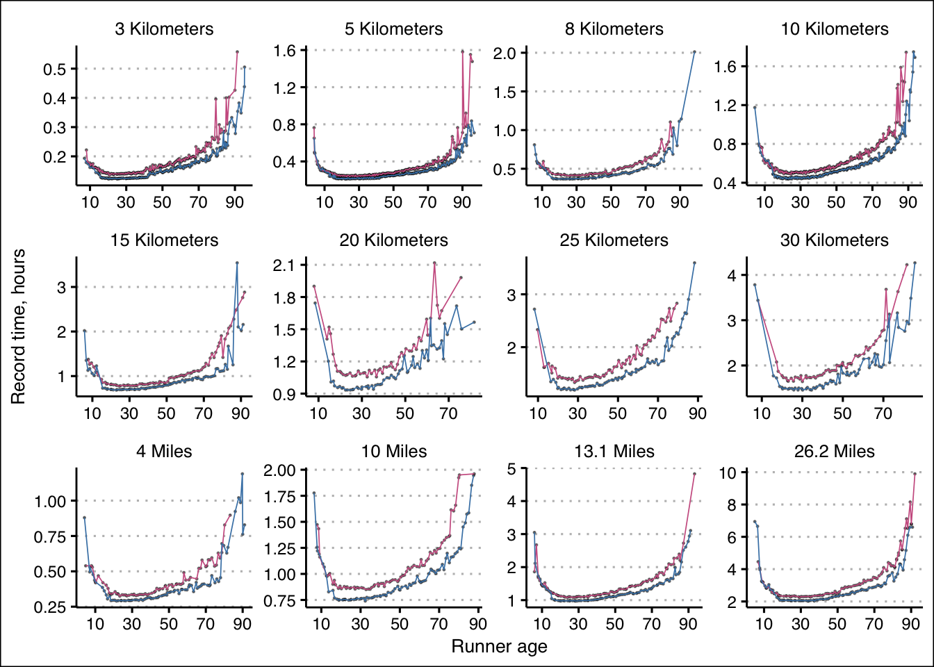
Let’s review the single-age record data for all race distances and gender:
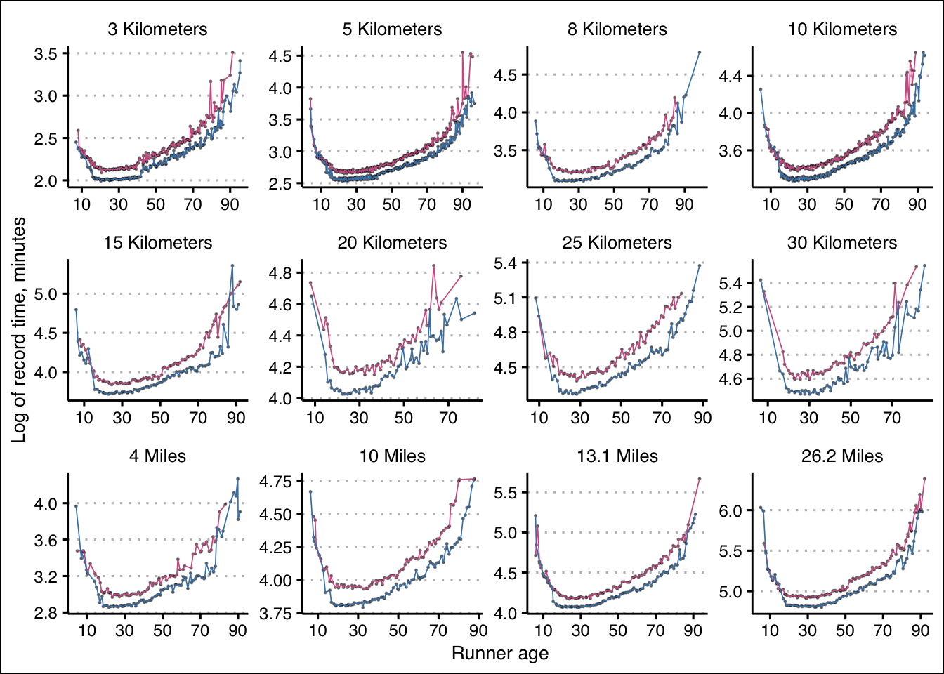
 Let’s also consider the log of those record run times to consider the rates of change:
Prior work
Fair and Kaplan (2018) focused on the performance of older athletes. They explored the biological limit of human running speeds by modeling record times at several distances as a function of age for those 40 years and older.
The authors compared multiple models: a linear-quadratic model, a non-parametric model, and both using the extreme value distribution. Justifying the linear-quadratic model, they theorized that may make sense as information suggested that for ages between around 40 and 70, the log of run times increase linearly with age (a constant rate of decline) and in later years, that rate of decline increases. The authors impose a few restrictions on this linear-quadratic model.
Linear-Quadratic Model
Summarising the authors’ linear-quadratic model, let’s let \(k\) be age of the runner who set the record, \(r_k\) be the log of the record time at age \(k\), and \(b_k\) be the unobserved biological limit for the log of the record run time at age \(k\). The biological limit is related to the record run time in that the record \(r_k\) is some \(\epsilon\) amount above \(b_k\):
\[ r_k = b_k + \epsilon_k \] The biological limit, in turn, is a linear function of age up to an unobserved threshold \(k^*\) and afterwards becomes a quadratic function of age:
\[ b_k = \begin{cases} \beta + \alpha k, &\quad 40 \le k \le k^*, \quad \alpha > 0 \\ \gamma + \theta k + \delta k^2, &\quad k > k^*, \quad \delta > 0 \end{cases} \]
The two functions are restricted in the two must “touch” and have the same slope (first derivative) at \(k^*\); thus,
\[ \gamma = \beta + \delta k^{*2}, \\ \theta = \alpha - 2 \delta k^* \] If we perform variable substitutions,
\[ b_k = \begin{cases} \beta + \alpha k, &\quad 40 \le k \le k^*, \quad \alpha > 0 \\ \beta + \delta k^{*2} + (\alpha - 2 \delta k^{*}) k + \delta k^2, &\quad k > k^*, \quad \delta > 0 \end{cases} \]
and simplify,
\[ \beta + \delta k^{*2} + \alpha k - 2 \delta k^{*} k + \delta k^2, \quad k > k^*, \quad \delta > 0 \]
we obtain this final form:
\[ \beta + \alpha k + \delta (k^{*2} - 2 k^{*} k + k^2), \quad k > k^*, \quad \delta > 0 \]
Non-parametric model
Fair and Kaplan (2018) also explore a non-parametric model, restricted in that the first and second derivatives must be nonnegative and nondecreasing. Here, I’ll relax these restrictions for modeling, though for the given data, those restrictions would hold.
Extreme value theory
The above models, as the authors note, finds the expected value of the records as a function of age. But with using extreme value theory, we can statistically estimate the true biological limit. The probability density corresponding to a given observed record \(r_k\) is
\[ f_{R_k}(r_k) = \eta \lambda (r_k - b_k) ^ {\lambda - 1} e^{-\eta (r_k - b_k)^{\lambda}} \] where I specify \(b_k\) as either the above linear-quadratic or nonparametric model.
Analysis
Of note, a review of Figure ?? above suggests that a linear model doesn’t quite fit what the data suggest (the rate of change does not quite appear to be constant even early on). Regardless, we’ll begin with a model similar to the linear-quadratic model described in Fair and Kaplan (2018).
We’ll use Stan for modeling estimates. For an initial analysis, let’s focus on 5K run times for male athletes aged 40 and over. For our linear-quadratic model, let’s remove from the data what Fair and Kaplan (2018) call “soft observations”; i.e., observed records at a given age that is slower than any record by an older runner:
data {
  int<lower=0> N;
  vector<lower=0>[N] rk_log;
  array[N] int<lower=0> k;
}

parameters {
  real beta;
  real<lower=0> alpha;
  real<lower=0> delta;
  real<offset=70, multiplier=10> k_star;
  real<lower=0> sigma;
}

model {
  beta   ~ std_normal();
  alpha  ~ exponential(1);
  delta  ~ exponential(1);
  sigma  ~ exponential(1);
  k_star ~ normal(70, 10);

  vector[N] mu;

  for( i in 1:N) mu[i] = beta + alpha * k[i] +
  (k[i] > k_star ? delta * (k_star ^ 2 - 2 * k_star * k[i] + k[i] ^ 2) : 0);

  rk_log ~ normal(mu, sigma);
}

generated quantities {
  vector[N] rk_log_hat;

  for( i in 1:N)
    rk_log_hat[i] = normal_rng(
    beta + alpha * k[i] + (k[i] > k_star ?
      delta * (k_star ^ 2 - 2 * k_star * k[i] + k[i] ^ 2) : 0), sigma);
}
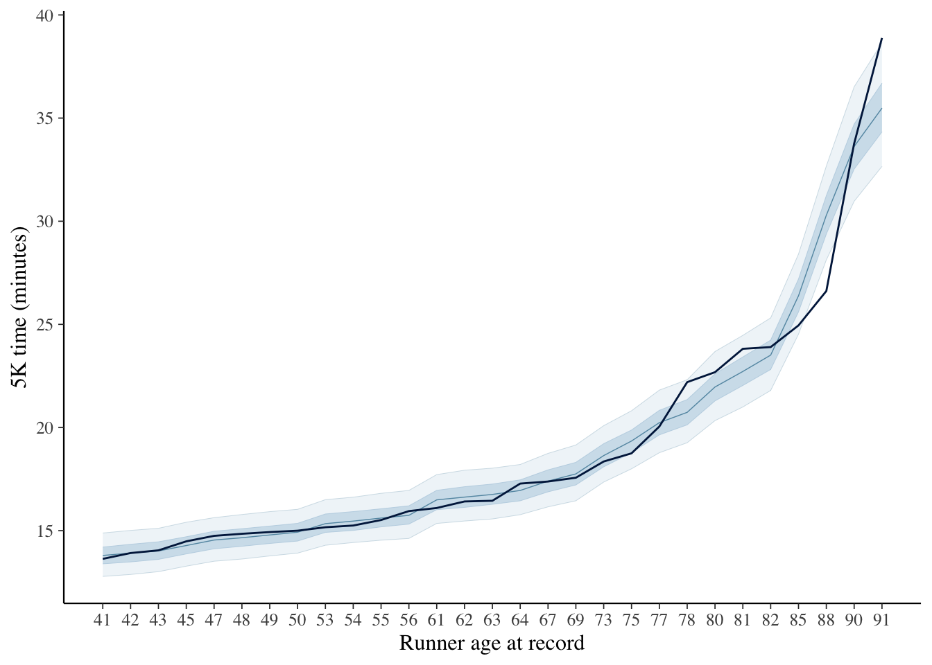
We should probably use more information to set more informative priors. For now, thoug, let’s compare the resulting expectations, conditional on the model and data, with the observed records:
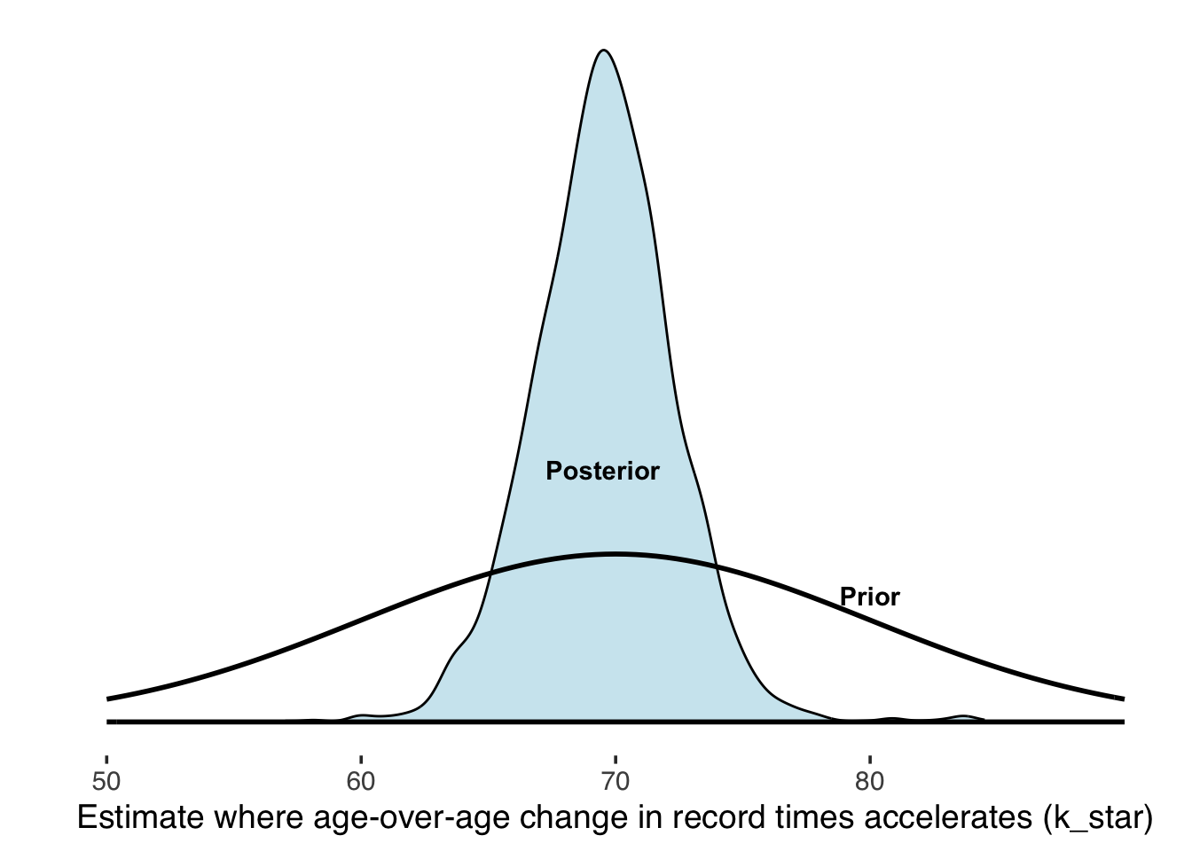
 Our posterior estimate for the age where age-over-age change in record times begins to accelerate is around 70, not moving much from our prior’s location, but the data add support by concentrating closer to 70:
Next, let’s consider a nonparametric model based on extreme value theory. Here’s it is, where the biological minimum \(b_k\) is a fraction of the record \(r_k\):
data {
  int<lower=0> N;
  vector<lower=0>[N] rk;
  array[N] int<lower=0> k;
}

parameters {
  vector<lower=0, upper=1>[N] b_;
  real<lower=0> kappa;
  real<lower=0> lambda;
}

transformed parameters {
  vector[N] b = b_ .* rk;
}

model {
  b_ ~ beta(20, 1.5);
  kappa ~ exponential(1);
  lambda ~ exponential(1);

  rk - b ~ weibull(kappa, lambda);
}

generated quantities {
  vector[N] rk_hat =
    rk - to_vector(weibull_rng(rep_vector(kappa, N), rep_vector(lambda, N)));
}
Conditional on this model and data, here are the expectations of the biological envelope, overlain again with the observed records:
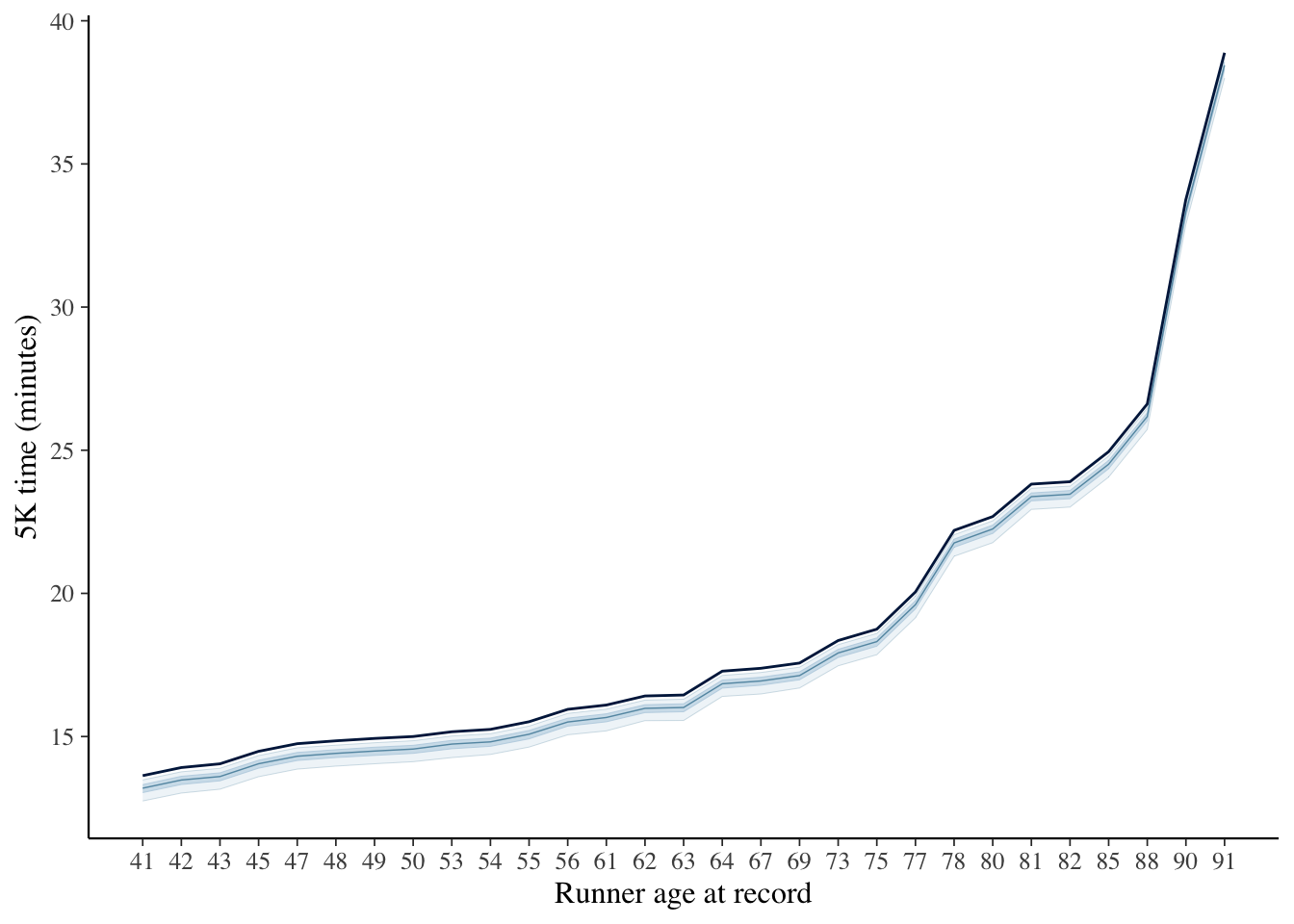
Of note, in this case, I only modeled parameters for ages with data. The estimation of a biological minimum are at and below the trend line of observed records. The estimates, below, of our biological limit \(b_k\) as a fraction of record times are less than 10 percent faster, the uncertainty of which is shown below using the first 200 draws from our model:
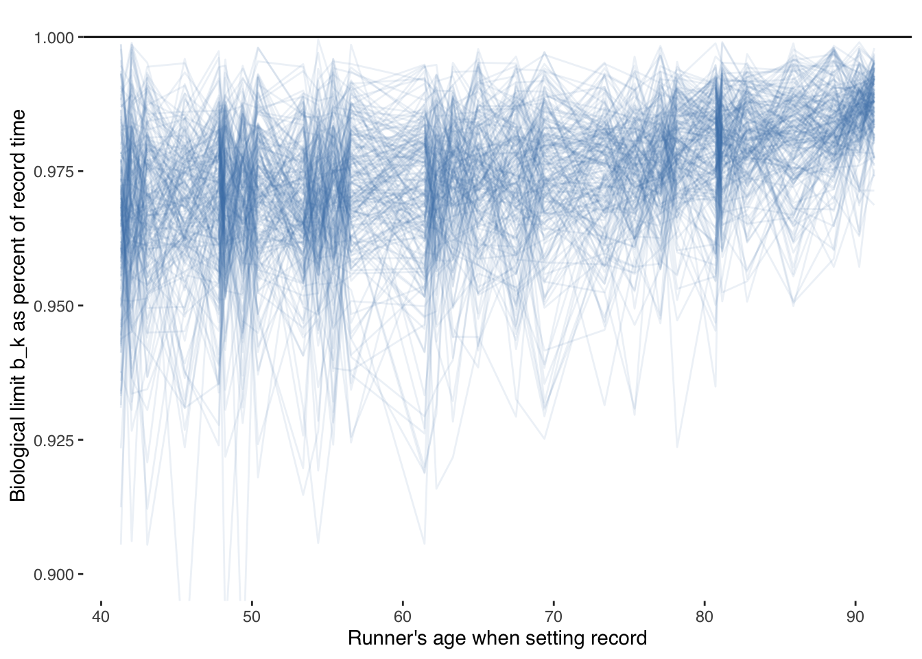
It seems odd that the biological limit would approach the record times as age increases since there are fewer older humans attempting those records.
In a later post, I’ll continue the analysis and, among other things, compare another form of modeling, bring in additional data, and, unlike Fair and Kaplan (2018), account for those “soft observations” instead of simply removing them. With each extension to this analysis, we should learn a little more about what Prefontaine set out to test: the limits of the human heart.