Modeling Umpire Calls
Introduction
The goal of baseball pitchers — when contributing to team defense — is to put out batters. Two ways are (mostly) within the pitchers’ control. They may earn a called strike or a swinging strike. The “definition of a good pitcher”, explains Sandy Koufax, is a “guy that throws what he intends to throw.” (Morrison, Pavlidis, and Long 2018) said that quantifying pitchers’ abilities to “throw the ball where he intends to”, called pitching command, is “one of the most challenging aspects of pitching to quantify.” As data of where the pitcher “intends to” throw are not publicly available, we agree. Various approaches have been tried. Baseball Info Solutions has measured catcher mitt starting locations for each pitch (Dewan 2011), to which ball catch locations are compared. But pitchers are not necessarily aiming at the mitt: consider catcher mitt location, for example, when a ball curves through the strike zone before diving into the dirt.
Trying another approach, (Morrison, Pavlidis, and Long 2018) “identified target points in each corner of the zone using the likelihood of a pitch to be called a strike, and quantify the pitcher’s ability to hit that spot consistently.” The authors divided “the strike zone into quadrants that highlight a pitcher’s ability to miss the most dangerous part of the zone. These quadrants are mapped against Called Strike Probability . . . contours to identify the ideal target in each section of the zone.”
This approach seems partly an improvement to the extent it considers probabilities of called strikes (called strike probabilities were not directly estimated, discussed later). But a static, target point in four quadrants inside the strike zone, defined without context of each at bat, are even less an intended target than the mitt. Pitching intentions are described by Don Drysdale,
When the ball is over the middle of the plate, the batter is hitting it with the sweet part of the bat. When it’s inside, he’s hitting it with the part of the bat from the handle to the trademark. When it’s outside, he’s hitting it with the end of the bat. You’ve got to keep the ball away from the sweet part of the bat. To do that, the pitcher has to move the hitter off the plate.
Instead of trying to measure pitcher command to the mitt or a few static points, we can assume the pitcher intends to maximize the probability of ideal outcomes: called or swinging strikes. That means pitching with movements to locations — continuous regions — that maximize probabilities of ideal outcomes. We aim to model ideal outcomes,
\[\begin{equation} p(\textrm{ideal outcome})=p(\textrm{called strike}) \cdot (1 - p(\textrm{swing})) + p(\textrm{whiff}\mid \textrm{swing}) \cdot p(\textrm{swing}) \tag{1} \end{equation}\]where these probabilities are modelled generatively. With such a model, we can explore questions such as whether consistency in pitching for ideal outcomes varies for starting pitchers as pitch counts pile up.
Batting and pitching data from Major League Baseball Advance Media
For modeling, we start with MLBAM’s publicly available information of all games from the 2017 regular season. An early, concise description of these data are available in (Fast 2007).
These data are transformed and cleaned in several ways. Pitch location measurements are converted to inches. The vertical locations are centered to the middle of each batter’s strike zone, which is defined in the rules of baseball,
The STRIKE ZONE is that area over home plate the upper limit of which is a horizontal line at the midpoint between the top of the shoulders and the top of the uniform pants, and the lower level is a line at the hollow beneath the kneecap. The Strike Zone shall be determined from the batter’s stance as the batter is prepared to swing at a pitched ball.
(MLB 2017). The top and bottom of the zone depend on player anatomies and are judged each pitch. Take note of both the inherent uncertainty and pitch-by-pitch variation: the “Strike Zone shall be determined from the batter’s stance as the batter is prepared to swing at a pitched ball.” Some variation exists in the strike zone, even for a given batter as we do not expect his stance to remain constant.
Along with batter stance variation, the per-pitch strike zone measurements have error (Lemire 2017) and include values too extreme to be possible, as shown in Table 1.
| variable | missing | complete | mean | sd | p0 | p25 | p50 | p75 | p100 |
|---|---|---|---|---|---|---|---|---|---|
| sz_bot | 0 | 436988 | 18.6 | 1.72 | -44.36 | 17.61 | 18.76 | 19.68 | 76.89 |
| sz_top | 0 | 436988 | 40.88 | 2.43 | -7.89 | 39.42 | 40.93 | 42.44 | 109.89 |
We supplement these data using prior information. Controlled, anatomical measures of male soldiers have been published by the United States Military (Benson and Parham 2017). Presumably anatomical measurements of male soldiers approximate the stature of pro ball players. These data, shown in Figure 1, include overall, knee (mid-patella), and navel height (Gordon et al. 2014), which should be close to the defined zone as seen by umpires.

Figure 1: Anthropological survey of male anatomies
MLBAM zone measurements more than three standard deviations outside the anatomical data corresponding to each batter’s height are recoded as missing and replaced by the mean of measurements from the same batter heights in the study. Post-cleaned medians and standard deviations of within-batter, per-pitch measurements of the bottom and top of their strike zones are shown in Table 2.
| variable | missing | complete | mean | sd | p0 | p25 | p50 | p75 | p100 |
|---|---|---|---|---|---|---|---|---|---|
| Median Bottom Strike Zone | 0 | 893 | 19.72 | 0.93 | 17.28 | 19.07 | 19.7 | 20.4 | 22.62 |
| Median Top Strike Zone | 0 | 893 | 43 | 1.72 | 37.32 | 41.83 | 42.84 | 44.1 | 47.88 |
| Standard Deviation Bottom Strike Zone | 22 | 871 | 0.65 | 0.28 | 0 | 0.58 | 0.7 | 0.79 | 2.18 |
| Standard Deviation Top Strike Zone | 22 | 871 | 0.92 | 0.41 | 0 | 0.8 | 1.02 | 1.16 | 2.51 |
| Within batter observations | 0 | 893 | 208.28 | 234.89 | 1 | 17 | 89 | 368 | 1021 |
Post-cleaning measurements of the strike zone and pitch locations on called strikes for players José Altuve and Aaron Judge, for perspective, are shown in Figure 2 alongside a sketch for context of their relative heights.

Figure 2: Post-cleaning measurements of the strike zone with called strike locations measured in inches (umpire’s view)
While called strikes are spread fairly throughout Altuve’s (varied) zone(s), relatively few called strikes are near the upper region of Judge’s zone(s) and significant numbers are below. For our model, post-cleaned median values per batter are used to approximate each batter’s strike zone, ignoring within-batter measurement error and variation. (Examples of more sophisticated approaches to measurement error are described in (Stan Development Team 2017), (Muff et al. 2015), and (McElreath 2015).) These data are filtered to keep only umpire calls on balls and strikes. The working model is used to estimate per-pitch probabilities of called strikes.
Modeling called strike probabilities is part of our larger goals, reconsidering measures of pitching command and exploring trends and variation as games progress. As such, any games for which no data were available from the beginning of the game were removed. We also identify whether (1) each pitch was the last pitch of the game (i.e., the data are censored), (2) the next batter stands opposite the pitcher’s throwing arm, and accumulations of (3) runs allowed, (4) homeruns, (5) runners on base, and (5) outs after each pitch. These data are used later in the analysis.
Modeling called strike probabilities
Called strikes by definition depend on pitched ball locations at home plate relative to that batter’s strike zone. Our data for modeling probabilities of called strikes are listed in Tables 3 to 5.
| variable | missing | complete | n | min | max | empty | n_unique |
|---|---|---|---|---|---|---|---|
| des | 0 | 185995 | 185995 | 4 | 13 | 0 | 2 |
| gameday_link | 0 | 185995 | 185995 | 30 | 30 | 0 | 2428 |
| variable | missing | complete | n_unique | top_counts |
|---|---|---|---|---|
| batter | 0 | 185995 | 893 | 572: 1021, 605: 923, 455: 915, 458: 913 |
| stand | 0 | 185995 | 2 | R: 108199, L: 77796, NA: 0 |
| umpire | 0 | 185995 | 92 | 521: 2899, 482: 2611, 427: 2529, 483: 2520 |
| variable | missing | complete | mean | sd | p0 | p25 | p50 | p75 | p100 |
|---|---|---|---|---|---|---|---|---|---|
| b_height | 0 | 185995 | 73.13 | 2.2 | 66 | 72 | 73 | 75 | 81 |
| px | 0 | 185995 | 0.5 | 10.64 | -20.5 | -8.37 | 0.9 | 9.4 | 20.5 |
| pz_centered | 0 | 185995 | -3.51 | 9.89 | -24.76 | -11.36 | -4.25 | 3.78 | 22.42 |
| sz_bot | 0 | 185995 | 19.69 | 1.07 | 16.19 | 18.9 | 19.61 | 20.45 | 26.2 |
| sz_top | 0 | 185995 | 42.8 | 1.81 | 36.3 | 41.57 | 42.84 | 44.1 | 52.64 |
| zone_ht | 0 | 185995 | 23.14 | 1.08 | 20.04 | 22.41 | 23.01 | 23.73 | 26.93 |
Previous work
Our modeling differs significantly from earlier work. (Brooks, Pavlidis, and Judge 2015)’s called strike probability model aims to assign “called strikes above average” to particular catchers (to measure their framing abilities) using a mixed-effects model. Their model does not directly estimate called strike probabilities from pitch location and other relevant variables. Instead, it includes as a parameter a “composite probability of a strike being called” obtained from Pitch Info Solutions. Pitch Info Solutions’s proprietary algorithm is said to include “a particular type of pitch in a particular location during a particular count at a particular ball park”. It is unclear whether the proprietary probabilities that (Brooks, Pavlidis, and Judge 2015) combine with player and umpire identity parameters are matched pitch-to-pitch. Their model is later used to examine pitching performance in (Pavlidis, Judge, and Long 2017) and (Morrison, Pavlidis, and Long 2018) but the underlying proprietary, composite called strike probabilities remain a predictor separate from their models.
Like (Brooks, Pavlidis, and Judge 2015), (Deshpande and Wyner 2017) explore catchers’ abilities to frame pitches and include, as an input to their model, a parameter for called strike probabilities. The authors helpfully compare the two approaches:
Rather than specifying a explicit parametrization in terms of the horizontal and vertical coordinates, we propose using a smoothed estimate of the historical log-odds of a called strike as an implicit parametrization of pitch location. This is very similar to the approach taken in (Brooks, Pavlidis, and Judge 2015), who included the estimated called strike probability as a covariate in their probit model.
(Deshpande and Wyner 2017) differ, however, in that they estimate their own called strike probabilities using four separate models, one for each combination of pitcher and batter handedness. In each, horizontal and vertical locations of the pitch are variables that interact within an undisclosed smoothing function in a generalized additive model. Curiously, these pitch location data are “historical”, and lack congruency with the data used as random effects parameters in their ultimate model.
General model description
The generative approach described here, in contrast with earlier work, explicitly models the underlying components defined in the rules of baseball, including batter anatomies and pitch locations. Per the rules, batter anatomies define the upper and lower bounds of each strike zone. (Deshpande and Wyner 2017) average the measurements from PITCHf/x on the top and bottom boundaries of the strike zone to show heatmaps of pitch locations. But this information was not used in their modeling of called strike probabilities. We do, as explained above. Further, we calculate the length of each batter’s zone as a parameter interacting with pitch location. Anticipating that batter handedness may affect umpire calls, we stratify the nonlinear, smoothing predictors for ball location by handedness.
Congruent with pitch location and zone length, our model also includes those making the calls — umpires! As mentioned, the strike zone requires a subjective judgment: was the ball above or below “the midpoint between the top of the shoulders and the top of the uniform pants”, for example, “as the batter is prepared to swing”? Considering the speed and movement of the ball and the timing needed to make this judgment, it is understandable that umpires apply the rules imperfectly (Lemire 2017). Some are better than others and technology has helped them become more consistently accurate (Davis and Lopez 2015). The particular home plate umpire and his calls, then, are part of our generative model. Earlier work suggests umpire calls are influenced by context, namely the ball-strike count (MacMahon and Starkes 2008), so we include count too.
To the extent that umpires’ perceptions of balls and strikes succumb to framing effects by catchers, see (Deshpande and Wyner 2017) and (Judge 2018), including catcher identities could improve this model. We also omit pitch type as the pitcher’s grip on the ball is hidden and modeling pitch types accurately are difficult, a task to be handled outside the scope here (MLBAM’s pitch classifications rely on a proprietary algorithm, not direct observation, and its accuracy can be improved. Some approaches have been explored in (Albert et al. 2017)).
Our model incorporates a spline function to estimate changes in the probability of a called strike with changes in pitched-ball location and batter strike zone length. Mathematically, our model can be written as,
\[\begin{equation} p(y_i = 1) = \textrm{logit}^{-1}(\alpha + \alpha_{j[i]} + \cdots + \mathcal{S}) \tag{2} \end{equation}\]where \(p(y_i = 1)\) is the probability that the umpire’s call \(y\) for pitch \(i\) is a strike. Probabilities are mapped from a logistic transformation1 of the predictors. We combine information on umpire decisions by pooling all calls together and jointly grouping those calls by umpire,
\[\begin{equation} \alpha_j \sim \textrm{N}(0, \sigma^2_j) \textrm{ for j = 1, ..., umpires} \tag{3} \end{equation}\]The information from each umpire’s calls depend upon the variance in their calls for observed pitches compared with the variance of calls for pitches pooled across the population of umpires. Variance for binary outcomes (called strike or not) are,
\[\begin{equation} \sigma_y = \sqrt{p (1 - p)} \tag{4} \end{equation}\]Thus, the amount of information for umpire \(j\) in the model is approximately,
\[\begin{equation} \alpha_{j} = \dfrac{\dfrac{n_j}{\sigma_y^2} \cdot \bar{y}_j + \dfrac{1}{\sigma_{\alpha}^2} \cdot y_{\mathrm{all}}}{\dfrac{n_j}{\sigma_y^2} + \dfrac{1}{\sigma_{\alpha}^2}} \tag{5} \end{equation}\]We parameterize pitch location and batter-specific zone length as,
\[\begin{equation} \mathcal{S}(\cdot) = \beta_1 + \beta_2x + \sum_{h=3}^{H+2}{\beta_hb_h(\cdot)} \tag{6} \end{equation}\]where the basis function \(b_h(\cdot)\) for the smoothing spline \(\mathcal{S}(\cdot)\) includes the horizontal and vertical location of each pitched ball at the vertical plane intersecting the front of home plate, along with the batter’s strike zone length. The particular spline chosen applies the same smoothing across these variables, which should be appropriate as they are isotropic and all measured in the same units (inches). The data used in this model are shared with the additional models for batter choice to swing and ability to make contact. As the probabilities of called strikes are presumably independent of batters’ decisions or abilities, however, we model umpire calls separately.
Called strike probabilities modeled in Stan
All models are coded using the Stan modeling language (Stan Development Team 2017), while data preparation and post-modeling analyses are coded in R. Some of the data are withheld from modeling for use in post-modeling checks. A random 30 percent of observations are withheld for testing.
We specified \(\textrm{normal}(0,1)\) across coefficients to provide some regularization, and \(\textrm{exponential}(1)\) across variance terms. When specifying the number of knots to create the smoothing splines, too few result in a probability model that doesn’t capture the underlying process while too many may result in overfitting. Somewhere around 60 seemed sufficient, give or take, after a bit of experimentation.2
The model specification includes,
\[\begin{equation} p(\textrm{call = strike}) \sim \textrm{ball-strike count} + \mathcal{S}(\textrm{x}, \textrm{z}_{\textrm{centered}}, \textrm{zone height}, \textrm{by = stand}, k = 60) + (1 \mid \textrm{umpires}) \tag{7} \end{equation}\]Model diagnostics
Our analysis follows the recommended Bayesian workflow (Gabry et al., n.d.). We next check the model for problems. All \(\hat{r}\) values are near 1.0, and \(\widehat{\textrm{neff}}\) sample sizes are substantial. Approximating leave-one-out cross-validation, reveals that some of the observations used for modeling have somewhat elevated (Vehtari, Gelman, and Gabry, n.d.) Pareto-K values, colored blue in Figure 3, which means those observations could have disproportionate influence on model parameters.
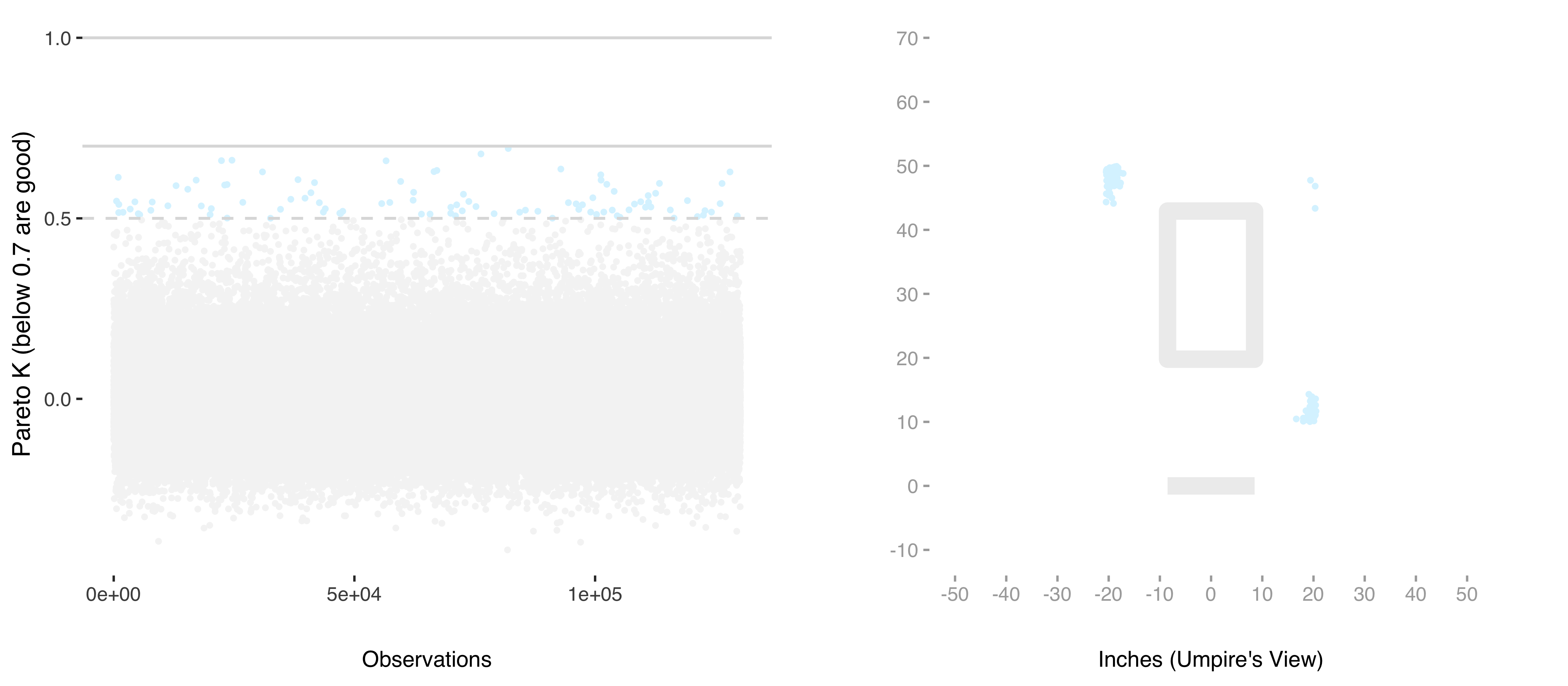
Figure 3: Diagnostics using PSIS-LOO approximation
These observations are well within the empirically accepted threshold and are several inches outside the average strike zone. We check the fit by binning residuals (Gelman et al. 2000, sec. 6.4) on the held-out data. Figure 4 shows observations binned in one tenth of a percent increments compared with one and two standard deviations of the binomial distribution.

Figure 4: Residuals binned by called strike probabilities of held-out data
Approximately 68.3 percent of the binned simulations fall within one standard deviation (the interior dashed lines), about what we expect, revealing no problems with under or over fitting. It is also a good sign that the binned residuals reveal no obvious patterns.
Called strike probability predictions from the modeled posterior
Our model’s estimates of called strike probabilities for right-handed batters are shown in Figure 5 overlaying a strike zone for the average player, and compared with probabilities for players seeing eye-to-eye with José Altuve and those taller, like Aaron Judge.

Figure 5: Posterior called strike probabilities by pitch location, measured in inches (umpire’s view)
The model seems plausible when comparing predictions with actual called strikes against Altuve and Judge (shown above, Figure 2). Umpires view each pitch with line-of-sight between the catcher and batter. From this perspective, we expect that umpires would have some difficulty with depth perception of pitches located low and outside. And this can be seen from the lack of symmetry in the model estimates. Also of note, the model suggests that on average umpires do not fully consider batter height when judging the zone. This model is folded into our larger model, described in a future post.
Bibliography
Albert, Jim, Mark E Glickman, Tim B Swartz, and Ruud H Koning. 2017. Handbook of Statistical Methods and Analyses in Sports. CRC Press.
Benson, Jane, and Joseph Parham. 2017. “For good measure – Natick releases raw data from Army-wide anthropometric survey.” https://www.army.mil/article/188601/for_good_measure_natick_releases_raw_data_from_army_wide_anthropometric_survey.
Brooks, Dan, Harry Pavlidis, and Jonathan Judge. 2015. “Moving Beyond WOWY: A Mixed Approach to Measuring Catcher Framing - Baseball Prospectus.” https://www.baseballprospectus.com/news/article/25514/moving-beyond-wowy-a-mixed-approach-to-measuring-catcher-framing/.
Davis, Noah, and Michael Lopez. 2015. “Umpires Are Less Blind Than They Used to Be.” https://fivethirtyeight.com/features/umpires-are-less-blind-than-they-used-to-be/.
Deshpande, Sameer, and Abraham Wyner. 2017. “SAFE2: A Hierarchical Model of Pitch Framing.” arXiv.org, April, 1–35.
Dewan, John. 2011. “Evaluating Pitcher Accuracy with Catcher Charting.” https://www.billjamesonline.com/stats290/?print=y.
Fast, Mike. 2007. “Glossary of the Gameday pitch fields.” https://fastballs.wordpress.com/2007/08/02/glossary-of-the-gameday-pitch-fields/.
Gabry, Jonah, Daniel Simpson, Aki Vehtari, Michael Betancourt, and Andrew Gelman. n.d. “Visualization in Bayesian workflow.” arXiv.org, 1–13.
Gelman, Andrew, Yuri Goegebeur, Francis Tuerlinckx, and Iven Van Mechelen. 2000. “Diagnostic Checks for Discrete Data Regression Models Using Posterior Predictive Simulations.” Applied Statistics 49 (2):247–68.
Gordon, Claire C, Cynthia L Blackwell, Bruce Bradtmiller, Joseph L Parham, Patricia Barrientos, Stephen P Paquette, Brian D Corner, et al. 2014. “2012 Anthropometric Survey of U.S. Army Personnel.” NATICK/TR-15/007.
Judge, Jonathan. 2018. “Bayesian Bagging to Generate Uncertainty Intervals: A Catcher Framing Story.” https://www.baseballprospectus.com/news/article/38289/bayesian-bagging-generate-uncertainty-intervals-catcher-framing-story/.
Lemire, Joe. 2017. “QuesTec’s Legacy, 20 Years Later: A Standard, Thinner, Lower Strike Zone.” https://www.sporttechie.com/questec-legacy-20-years-strike-zone/.
MacMahon, Clare, and Janet L Starkes. 2008. “Contextual influences on baseball ball-strike decisions in umpires, players, and controls.” Journal of Sports Sciences 26 (7):751–60.
McElreath, Richard. 2015. Statistical Rethinking. CRC Press.
MLB. 2017. “Official Baseball Rules 2017 Edition,” March, 1–284.
Morrison, Kate, Harry Pavlidis, and Jeff Long. 2018. “Pitching Scores: Power, Command, and Stamina.” https://www.baseballprospectus.com/news/article/37379/pitching-scores-power-command-stamina/.
Muff, Stefanie, Andrea Riebler, Leonhard Held, Hävard Rue, and Philippe Saner. 2015. “Bayesian analysis of measurement error models using integrated nested Laplace approximations.” Royal Statistical Society, Series C Applied Statistics 64 (2):231–52.
Pavlidis, Harry, Jonathan Judge, and Jeff Long. 2017. “Prospectus Feature: Command and Control.” Baseballprospectus.com, January.
Stan Development Team. 2017. Stan Modeling Language. 2.17.0 ed.
Vehtari, Aki, Andrew Gelman, and Jonah Gabry. n.d. “Practical Bayesian model evaluation using leave-one-out cross-validation and WAIC.” Statistics and Computing 27:1413–32.
Wood, Simon. 2017. Generalized Additive Models: an introduction with R. Second. CRC Press.