Milad Kharratzadeh provides a helpful case study on estimating splines in Stan. We can improve on his work with a few tricks to speed up the estimation process. Namely, if we decompose the spline matrix using QR decomposition, we speed up Stan’s fitting process by at least an order of magnitude.

Here’s how we can alter the code to accommodate splines with a few tricks to speed things up:

functions {
  
  vector build_b_spline(vector t, array[] real ext_knots, int ind, int order) {
    
    vector[size(t)] b_spline;
    vector[size(t)] w1 = rep_vector(0, size(t));
    vector[size(t)] w2 = rep_vector(0, size(t));
    
    if (order == 1)
    
      for (i in 1:size(t)) 
        b_spline[i] = (ext_knots[ind] <= t[i]) && (t[i] < ext_knots[ind+1]); 
    
    else {
    
      if (ext_knots[ind] != ext_knots[ind + order-1])
        w1 = (t - rep_vector(ext_knots[ind], size(t))) / 
             (ext_knots[ind + order-1] - ext_knots[ind]);
      if (ext_knots[ind + 1] != ext_knots[ind + order])
        w2 = 1 - (t - rep_vector(ext_knots[ind + 1], size(t))) / 
                 (ext_knots[ind + order] - ext_knots[ind + 1]);
                 
      b_spline = w1 .* build_b_spline(t, ext_knots, ind, order - 1) + 
                 w2 .* build_b_spline(t, ext_knots, ind+1, order - 1);
    
    }
    
    return b_spline;
  
  }
  
}


data {
  
  int<lower=1> T;                 // number of times measured
  vector[T] t;                    // remove and replace with position
  vector[T] y;                    // the measurement at each time point t
  
  int<lower=1> K;                 // number of knots
  int<lower=1> degree;            // degree of the spline
  int<lower=0,upper=1> penalized; // whether to use prior for smoothing
  
}


transformed data {
  
  // knots at evenly-spaced quantiles of data
  array[K] real p;
  for(i in 1:K) p[i] = (i - 1.0) / (K-1.0);
  array[K] real k = quantile(t, p);
  
  // build the spline matrix B
  int n_basis = K + degree - 1; 
  matrix[n_basis, T] B;
  
  array[2 * degree + K] real ext_knots =
  append_array(append_array(rep_array(k[1], degree), k), rep_array(k[K], degree));
  
  for (ind in 1:n_basis)
    B[ind,:] = to_row_vector(build_b_spline(t, (ext_knots), ind, degree + 1));
  
  B[K + degree - 1, T] = 1;
  
  // QR decomposition of B, thin and scale
  matrix[T, n_basis] Q_ast = qr_thin_Q(B') * sqrt(T - 1);
  matrix[n_basis, n_basis] R_ast = qr_thin_R(B') / sqrt(T - 1);
  matrix[n_basis, n_basis] R_ast_inverse = inverse(R_ast);
  
  // helper stuff
  vector[T] zeros_T = rep_vector(0, T);
  
}


parameters {
  
  vector[n_basis] theta_raw; // coefficients on Q_ast
  real<lower=0> sigma;       // scale of the variation
  real<lower=0> tau;         // penalization on wiggles
  
}


transformed parameters {
  
  vector[n_basis] theta;
  
  if(penalized) {
    theta[1] = theta_raw[1];
    for(i in 2:n_basis) theta[i] = theta[i-1] + theta_raw[i] * tau;
  } else {
    theta = theta_raw;
  }
  
}


model {
  
  theta_raw ~ normal(0, 1);
  tau ~ normal(0, 1);
  sigma ~ exponential(1);  
  y ~ normal_id_glm(Q_ast, zeros_T, theta, sigma);

}

generated quantities {
  vector[n_basis] beta;
  beta = R_ast_inverse * theta;
  vector[T] y_hat = B' * beta;
}

We can compile the model like so,

library(cmdstanr)
m = cmdstan_model('b_spline_QR.stan')

The main changes from the original case study are to decompose the spline matrix B into components:

  // QR decomposition of B
  matrix[T, n_basis] Q_ast;
  matrix[n_basis, n_basis] R_ast;
  matrix[n_basis, n_basis] R_ast_inverse;
  
  // thin and scale the QR decomposition
  Q_ast = qr_thin_Q(B') * sqrt(T - 1);
  R_ast = qr_thin_R(B') / sqrt(T - 1);
  R_ast_inverse = inverse(R_ast);

Then, we regress on the decomposed matrix.

Let’s simulate some data for the model and fit it:

set.seed(11)

num_knots <- 10
spline_degree <- 3
num_basis <- num_knots + spline_degree - 1

a0 <- 0.2
a <- rnorm(num_basis, 0, 1)

X <- seq(from=-10, to=10, by=.1)
knots <- unname(quantile(X,probs=seq(from=0, to=1, length.out = num_knots)))
num_data <- length(X)

B_true <- t(bs(X, df=num_basis, degree=spline_degree, intercept = TRUE))
Y_true <- as.vector(a0*X + a%*%B_true)
Y <- Y_true + rnorm(length(X), 0, 0.2)

With that data, let’s fit it in Stan using our improved model:

num_knots <- 20
spline_degree <- 3

dat <- list(
  T = length(X),
  K = num_knots,
  penalized = 1,
  degree = spline_degree,
  y = Y,
  t = X
)

fit <- m$sample(
  data = dat,
  parallel_chains = 4,
  iter_warmup = 500,
  iter_sampling = 500,
  adapt_delta = 0.8,
  max_treedepth = 9,
  refresh = 0
)

## Running MCMC with 4 parallel chains...
## 
## Chain 1 finished in 0.8 seconds.
## Chain 3 finished in 0.8 seconds.
## Chain 4 finished in 0.8 seconds.
## Chain 2 finished in 1.0 seconds.
## 
## All 4 chains finished successfully.
## Mean chain execution time: 0.9 seconds.
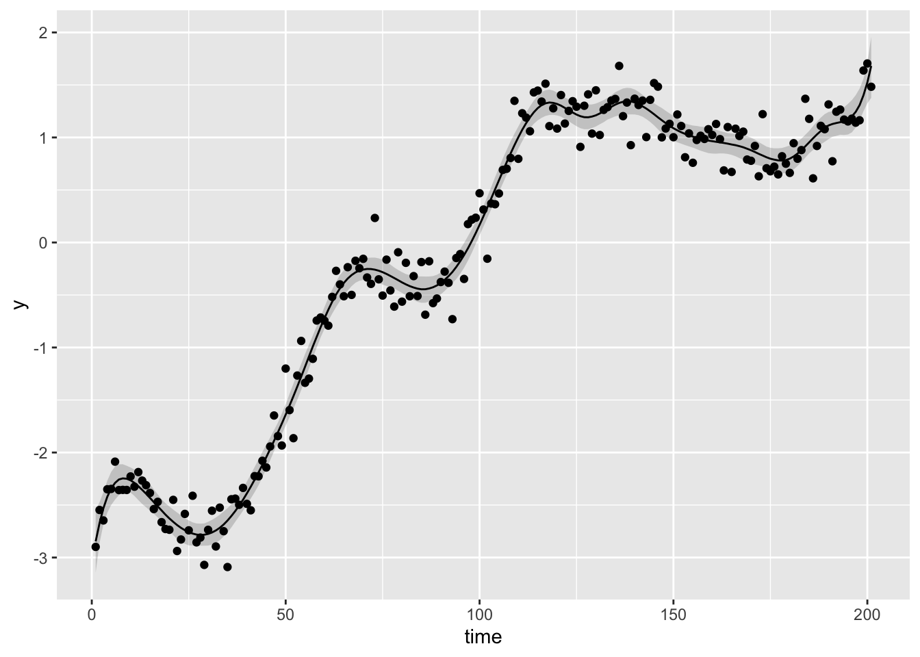
## Total execution time: 1.1 seconds.

Fast, nice! Here’s a look at our fit on the original simulated data:

yhat <- fit$summary('y_hat', ~quantile(., prob = c(0.025, 0.5, 0.975)))
x <- seq(nrow(yhat))

ggplot(yhat) + 
  geom_ribbon(
    mapping = aes(x, ymin = `2.5%`, ymax = `97.5%`), 
    alpha = 0.2
  ) + 
  geom_line(
    mapping = aes(seq(nrow(yhat)), y = `50%`)
  ) + 
  geom_point(
    mapping = aes(seq(nrow(yhat)), y = Y)
  ) + 
  labs(x = 'time', y = 'y')