Slide 35
In R, load libraries,
library(tidyverse)or in Python do the same,
import pandas as pd
from plotnine import *

from siuba.dply.vector import row_number, n, lag
from siuba import *
Slide 36
In R, import data from Citi Bike data storage if not available on your computer:
savefile <- "data/201901-citibike-tripdata.csv"

if (!file.exists(savefile)) {

  url <- str_c(
    "https://s3.amazonaws.com/tripdata/",
    "201901-citibike-tripdata.csv.zip"
  )

  download.file(url = url, destfile = savefile )

  }

df_r <- read_csv(savefile)
Let’s look at the beginning of the dataframe:
df_r %>% glimpse() Rows: 967,287
Columns: 15
$ tripduration <dbl> 320, 316, 591, 2719, 303, 535, 280…
$ starttime <dttm> 2019-01-01 00:01:47, 2019-01-01 0…
$ stoptime <dttm> 2019-01-01 00:07:07, 2019-01-01 0…
$ `start station id` <dbl> 3160, 519, 3171, 504, 229, 3630, 3…
$ `start station name` <chr> "Central Park West & W 76 St", "Pe…
$ `start station latitude` <dbl> 40.77897, 40.75187, 40.78525, 40.7…
$ `start station longitude` <dbl> -73.97375, -73.97771, -73.97667, -…
$ `end station id` <dbl> 3283, 518, 3154, 3709, 503, 3529, …
$ `end station name` <chr> "W 89 St & Columbus Ave", "E 39 St…
$ `end station latitude` <dbl> 40.78822, 40.74780, 40.77314, 40.7…
$ `end station longitude` <dbl> -73.97042, -73.97344, -73.95856, -…
$ bikeid <dbl> 15839, 32723, 27451, 21579, 35379,…
$ usertype <chr> "Subscriber", "Subscriber", "Subsc…
$ `birth year` <dbl> 1971, 1964, 1987, 1990, 1979, 1989…
$ gender <dbl> 1, 1, 1, 1, 1, 2, 1, 1, 2, 1, 1, 2…Of note, as of R 4.2, the base language includes a pipe operator |>, but I’ll continue to use %>% from the R package magrittr as it has more features.
In Python, load our data:
df_py = pd.read_csv("data/201901-citibike-tripdata.csv")As with R, let’s get some information on the data frame:
df_py.info()<class 'pandas.core.frame.DataFrame'>
RangeIndex: 967287 entries, 0 to 967286
Data columns (total 15 columns):
# Column Non-Null Count Dtype
--- ------ -------------- -----
0 tripduration 967287 non-null int64
1 starttime 967287 non-null object
2 stoptime 967287 non-null object
3 start station id 967269 non-null float64
4 start station name 967269 non-null object
5 start station latitude 967287 non-null float64
6 start station longitude 967287 non-null float64
7 end station id 967269 non-null float64
8 end station name 967269 non-null object
9 end station latitude 967287 non-null float64
10 end station longitude 967287 non-null float64
11 bikeid 967287 non-null int64
12 usertype 967287 non-null object
13 birth year 967287 non-null int64
14 gender 967287 non-null int64
dtypes: float64(6), int64(4), object(5)
memory usage: 110.7+ MBSlide 37
In R, let’s create a new variable that flags whether the bike was rebalanced.
df_r <- df_r %>% rename_all(function(x) gsub(' ', '_', x))


df_r <- df_r %>%
  filter(!is.na(start_station_id)) %>%
  arrange(starttime) %>%
  group_by(bikeid) %>%
  mutate(
    rebalanced = (row_number() > 1) & (start_station_id != lag(end_station_id))
  ) %>%
  ungroup()


df_r %>% pull(rebalanced) %>% table()
.
FALSE TRUE
937908 29361 In Python,
df_py = df_py.rename(lambda x: x.replace(' ', '_'), axis = 1)

df_py = df_py >> \
  filter( _.start_station_id.notnull() ) >> \
  arrange( _.starttime ) >> \
  group_by( _.bikeid ) >> \
  mutate(
    rebalanced = (row_number(_) > 1) & (_.start_station_id != _.end_station_id.shift(1) )
  ) >> \
  ungroup()

df_py.rebalanced.value_counts( dropna = False )
False 937908
True 29361
Name: rebalanced, dtype: int64Slide 38
In R,
ggplot(data = df_r) +
  geom_bar(
    mapping = aes(x = rebalanced),
    stat = 'count'
  )
In Python,
ggplot(df_py) + \
geom_bar(
    mapping = aes(x = 'rebalanced'),
    stat = 'count'
  )
<ggplot: (784757209)>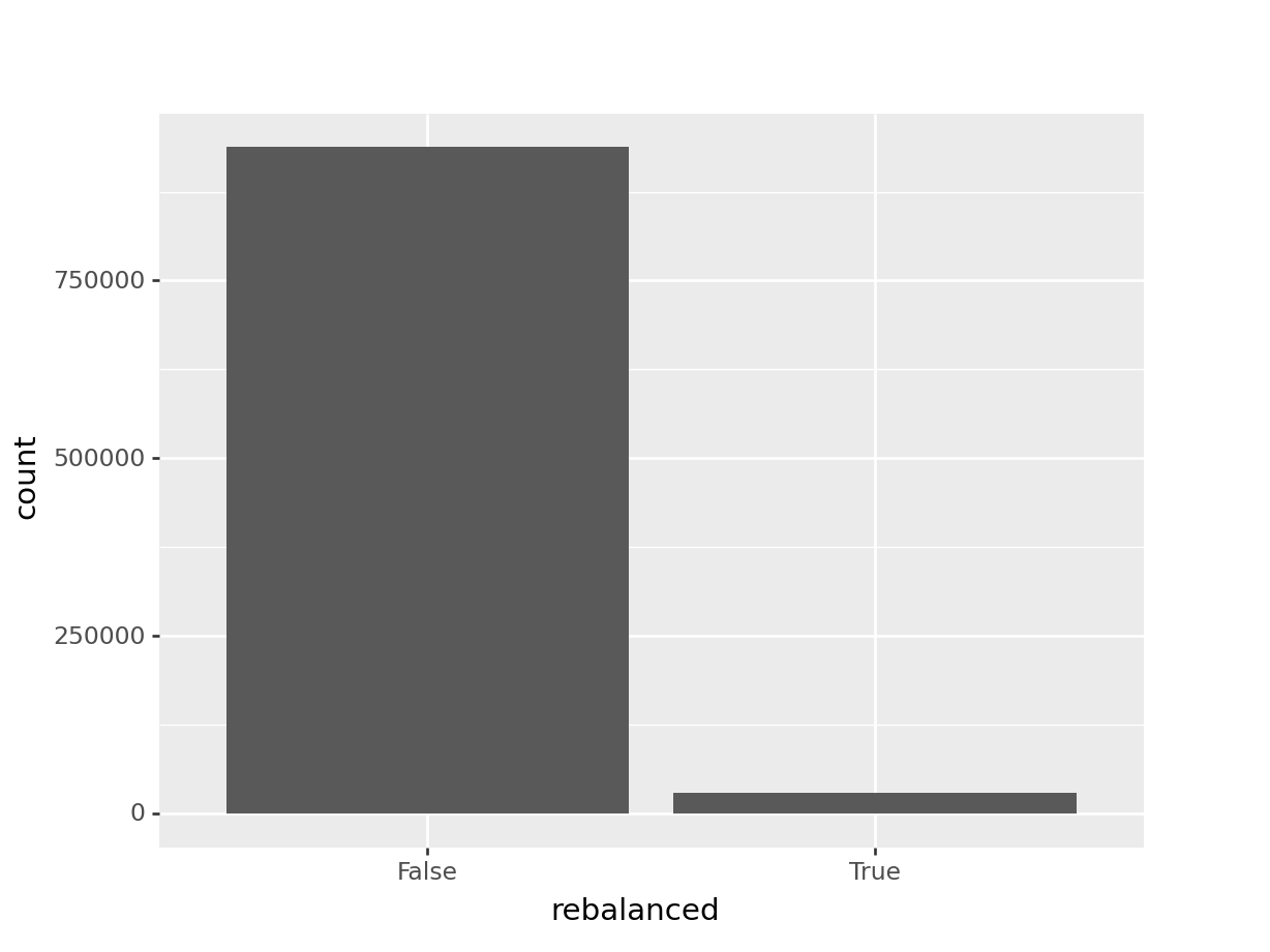
Slide 39
In R, we may code a simple linear regression using the base R function lm like so,
df_r <- df_r %>% mutate(gender_factor = factor(df_r$gender) )

model1 <- lm(
  formula = tripduration ~ rebalanced + gender_factor,
  data = df_r)

summary(model1)
Call:
lm(formula = tripduration ~ rebalanced + gender_factor, data = df_r)

Residuals:
    Min      1Q  Median      3Q     Max
  -1727    -443    -250      79 2678123

Coefficients:
               Estimate Std. Error t value Pr(>|t|)
(Intercept)     1717.67      38.69  44.401   <2e-16 ***
rebalancedTRUE    70.10      42.34   1.656   0.0978 .
gender_factor1 -1005.53      39.56 -25.418   <2e-16 ***
gender_factor2  -883.02      41.74 -21.153   <2e-16 ***
---
Signif. codes:  0 '***' 0.001 '**' 0.01 '*' 0.05 '.' 0.1 ' ' 1

Residual standard error: 7142 on 967265 degrees of freedom
Multiple R-squared:  0.0006904, Adjusted R-squared:  0.0006873
F-statistic: 222.7 on 3 and 967265 DF,  p-value: < 2.2e-16
and a generalized linear model using the base R function glm:
model2 <- glm(
  formula = rebalanced ~ tripduration + gender_factor,
  data = df_r,
  family = binomial())

summary(model2)
Call:
glm(formula = rebalanced ~ tripduration + gender_factor, family = binomial(),
    data = df_r)

Deviance Residuals:
    Min       1Q   Median       3Q      Max
-0.6669  -0.2421  -0.2419  -0.2419   2.6632

Coefficients:
                 Estimate Std. Error  z value Pr(>|z|)
(Intercept)    -3.459e+00  3.148e-02 -109.885  < 2e-16 ***
tripduration    7.722e-07  4.930e-07    1.566   0.1172
gender_factor1 -5.771e-02  3.224e-02   -1.790   0.0735 .
gender_factor2  1.610e-01  3.364e-02    4.787 1.69e-06 ***
---
Signif. codes:  0 '***' 0.001 '**' 0.01 '*' 0.05 '.' 0.1 ' ' 1

(Dispersion parameter for binomial family taken to be 1)

    Null deviance: 263044  on 967268  degrees of freedom
Residual deviance: 262799  on 967265  degrees of freedom
AIC: 262807

Number of Fisher Scoring iterations: 6
In Python, we can calculate the same models using the statsmodels library. Here’s the linear model:
import statsmodels.api as sm
import statsmodels.formula.api as smf

df_py = df_py >> mutate(gender_factor = _.gender.astype('category') )

model1 = smf.ols(
  formula = 'tripduration ~ rebalanced + gender_factor',
  data = df_py).fit()

model1.summary()
<class 'statsmodels.iolib.summary.Summary'>
"""
OLS Regression Results
==============================================================================
Dep. Variable: tripduration R-squared: 0.001
Model: OLS Adj. R-squared: 0.001
Method: Least Squares F-statistic: 222.7
Date: Wed, 19 Apr 2023 Prob (F-statistic): 1.82e-144
Time: 16:07:26 Log-Likelihood: -9.9559e+06
No. Observations: 967269 AIC: 1.991e+07
Df Residuals: 967265 BIC: 1.991e+07
Df Model: 3
Covariance Type: nonrobust
======================================================================================
coef std err t P>|t| [0.025 0.975]
--------------------------------------------------------------------------------------
Intercept 1717.6662 38.685 44.401 0.000 1641.844 1793.488
rebalanced[T.True] 70.0968 42.336 1.656 0.098 -12.880 153.074
gender_factor[T.1] -1005.5329 39.561 -25.418 0.000 -1083.070 -927.995
gender_factor[T.2] -883.0192 41.744 -21.153 0.000 -964.835 -801.203
==============================================================================
Omnibus: 4618545.968 Durbin-Watson: 2.000
Prob(Omnibus): 0.000 Jarque-Bera (JB): 94837513248820.281
Skew: 183.793 Prob(JB): 0.00
Kurtosis: 48510.579 Cond. No. 12.0
==============================================================================
Notes:
[1] Standard Errors assume that the covariance matrix of the errors is correctly specified.
"""and here’s the generalized linear model,
model2 = smf.glm(
  formula = 'rebalanced ~ tripduration + gender_factor',
  data = df_py,
  family = sm.families.Binomial() ).fit()

model2.summary()
<class 'statsmodels.iolib.summary.Summary'>
"""
Generalized Linear Model Regression Results
=====================================================================================================
Dep. Variable: ['rebalanced[False]', 'rebalanced[True]'] No. Observations: 967269
Model: GLM Df Residuals: 967265
Model Family: Binomial Df Model: 3
Link Function: Logit Scale: 1.0000
Method: IRLS Log-Likelihood: -1.3140e+05
Date: Wed, 19 Apr 2023 Deviance: 2.6280e+05
Time: 16:07:27 Pearson chi2: 9.67e+05
No. Iterations: 7 Pseudo R-squ. (CS): 0.0002534
Covariance Type: nonrobust
======================================================================================
coef std err z P>|z| [0.025 0.975]
--------------------------------------------------------------------------------------
Intercept 3.4594 0.031 109.885 0.000 3.398 3.521
gender_factor[T.1] 0.0577 0.032 1.790 0.073 -0.005 0.121
gender_factor[T.2] -0.1610 0.034 -4.787 0.000 -0.227 -0.095
tripduration -7.722e-07 4.93e-07 -1.566 0.117 -1.74e-06 1.94e-07
======================================================================================
"""