1. Storytelling with data

Example code used in class discussion.

Here is this code’s rmd file.

Slide 38

In R, load libraries,

library(tidyverse)

Slide 39

then import data:

df_r <- read_csv("data/201901-citibike-tripdata.csv")

Let’s look at the beginning of the dataframe:

df_r %>% glimpse() 

Rows: 967,287
Columns: 15
$ tripduration              <dbl> 320, 316, 591, 2719, 303, 535, 280…
$ starttime                 <dttm> 2019-01-01 00:01:47, 2019-01-01 0…
$ stoptime                  <dttm> 2019-01-01 00:07:07, 2019-01-01 0…
$ `start station id`        <dbl> 3160, 519, 3171, 504, 229, 3630, 3…
$ `start station name`      <chr> "Central Park West & W 76 St", "Pe…
$ `start station latitude`  <dbl> 40.77897, 40.75187, 40.78525, 40.7…
$ `start station longitude` <dbl> -73.97375, -73.97771, -73.97667, -…
$ `end station id`          <dbl> 3283, 518, 3154, 3709, 503, 3529, …
$ `end station name`        <chr> "W 89 St & Columbus Ave", "E 39 St…
$ `end station latitude`    <dbl> 40.78822, 40.74780, 40.77314, 40.7…
$ `end station longitude`   <dbl> -73.97042, -73.97344, -73.95856, -…
$ bikeid                    <dbl> 15839, 32723, 27451, 21579, 35379,…
$ usertype                  <chr> "Subscriber", "Subscriber", "Subsc…
$ `birth year`              <dbl> 1971, 1964, 1987, 1990, 1979, 1989…
$ gender                    <dbl> 1, 1, 1, 1, 1, 2, 1, 1, 2, 1, 1, 2…

In Python, load libraries,

import pandas as pd
from plotnine import *
from datar.all import *

from pipda import options
options.assume_all_piping = True

then load our data:

df_py = pd.read_csv("data/201901-citibike-tripdata.csv")

As with R, let’s get some information on the data frame:

df_py.info()

<class 'pandas.core.frame.DataFrame'>
RangeIndex: 967287 entries, 0 to 967286
Data columns (total 15 columns):
 #   Column                   Non-Null Count   Dtype  
---  ------                   --------------   -----  
 0   tripduration             967287 non-null  int64  
 1   starttime                967287 non-null  object 
 2   stoptime                 967287 non-null  object 
 3   start station id         967269 non-null  float64
 4   start station name       967269 non-null  object 
 5   start station latitude   967287 non-null  float64
 6   start station longitude  967287 non-null  float64
 7   end station id           967269 non-null  float64
 8   end station name         967269 non-null  object 
 9   end station latitude     967287 non-null  float64
 10  end station longitude    967287 non-null  float64
 11  bikeid                   967287 non-null  int64  
 12  usertype                 967287 non-null  object 
 13  birth year               967287 non-null  int64  
 14  gender                   967287 non-null  int64  
dtypes: float64(6), int64(4), object(5)
memory usage: 110.7+ MB

Slide 40

In R, let’s create a new variable that flags whether the bike was rebalanced.

df_r <- df_r %>% rename_all(function(x) gsub(" ", "_", x))


df_r <- df_r %>%
  filter(!is.na(start_station_id)) %>%
  arrange(starttime) %>%
  group_by(bikeid) %>%
  mutate(
    rebalanced = 
      if_else(row_number() > 1 & 
             start_station_id != lag(end_station_id),
             TRUE, FALSE)
  ) %>%
  ungroup()


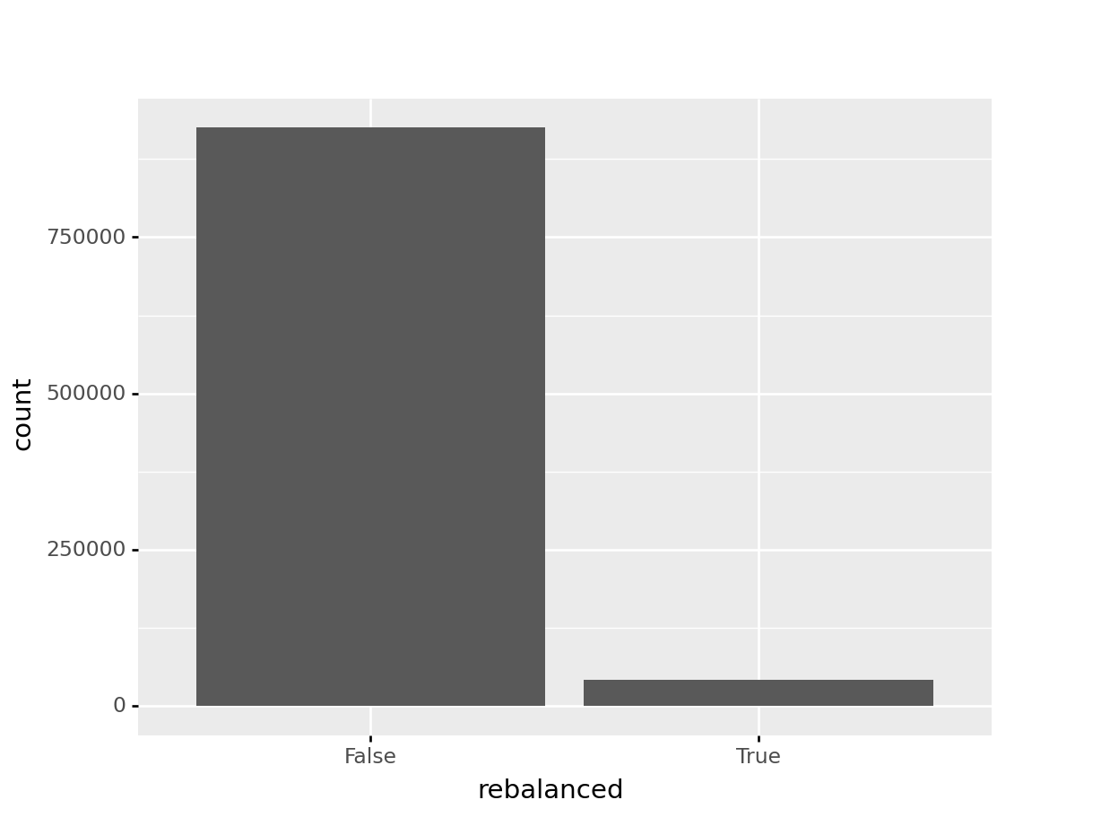
df_r %>% pull(rebalanced) %>% table()

.
 FALSE   TRUE 
937908  29361 

In Python,

df_py = df_py.rename(lambda x: x.replace(' ', '_'), axis = 1)


df_py = df_py >> \
  filter( f.start_station_id.notnull() ) >> \
  arrange(f.starttime) >> \
  group_by(f.bikeid) >> \
  mutate(
    rebalanced = if_else(
      (row_number() > 1) and 
      (f.start_station_id != lag(f.end_station_id)), 
      TRUE, FALSE) ) >> \
  ungroup()


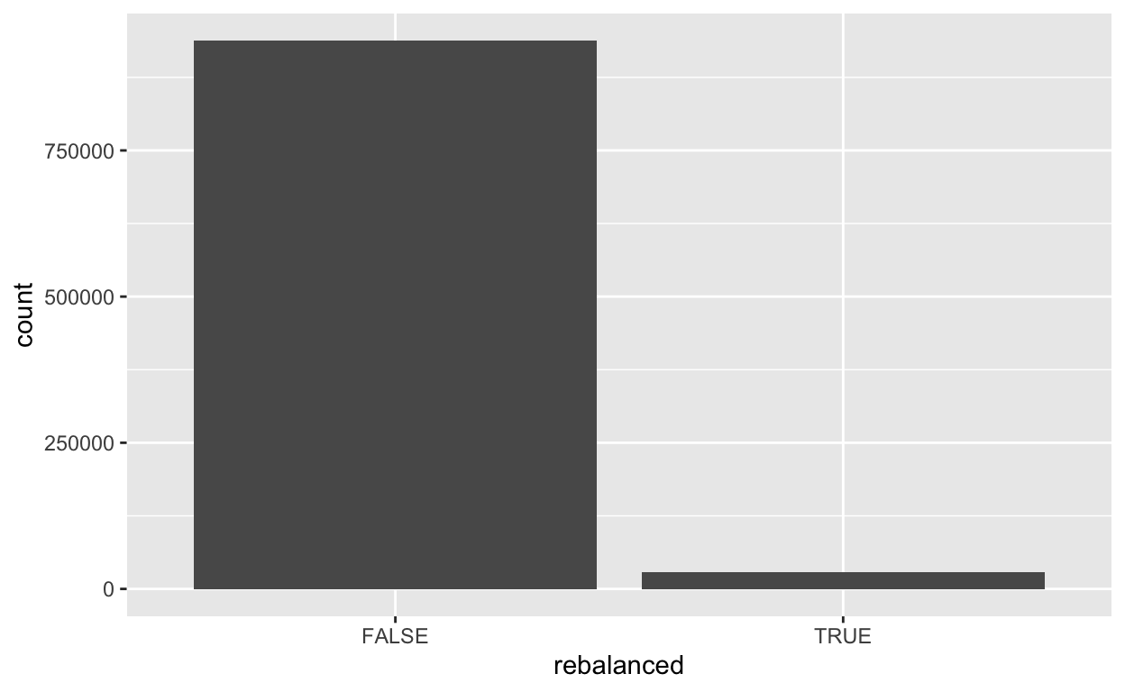
df_py.rebalanced.value_counts()

False    925273
True      41996
Name: rebalanced, dtype: int64

Slide 41

In R,

ggplot(data = df_r) + 
  geom_bar(
    mapping = aes(x = rebalanced), 
    stat = 'count'
  )

In Python,

ggplot(df_py) + \
geom_bar(
    mapping = aes(x = 'rebalanced'), 
    stat = 'count'
  )

<ggplot: (776427133)>