1. Storytelling with data

Example code used in class discussion.

Note, I’ve turned off (see eval=FALSE) in python code chunks below in case you have not installed python.

Slide 35

In R, load libraries,

library(tidyverse)

or in Python do the same,

import pandas as pd
from plotnine import *

from siuba.dply.vector import row_number, n, lag
from siuba import *

Slide 36

In R, import data from Citi Bike data storage if not available on your computer:

savefile <- "data/201901-citibike-tripdata.csv"

if (!file.exists(savefile)) {
  
  url <- str_c(
    "https://s3.amazonaws.com/tripdata/",
    "201901-citibike-tripdata.csv.zip"
  )
  
  download.file(url = url, destfile = savefile )
  
  }

df_r <- read_csv(savefile)

Let’s look at the beginning of the dataframe:

df_r %>% glimpse() 

Rows: 967,287
Columns: 15
$ tripduration              <dbl> 320, 316, 591, 2719, 303, 535, 280…
$ starttime                 <dttm> 2019-01-01 00:01:47, 2019-01-01 0…
$ stoptime                  <dttm> 2019-01-01 00:07:07, 2019-01-01 0…
$ `start station id`        <dbl> 3160, 519, 3171, 504, 229, 3630, 3…
$ `start station name`      <chr> "Central Park West & W 76 St", "Pe…
$ `start station latitude`  <dbl> 40.77897, 40.75187, 40.78525, 40.7…
$ `start station longitude` <dbl> -73.97375, -73.97771, -73.97667, -…
$ `end station id`          <dbl> 3283, 518, 3154, 3709, 503, 3529, …
$ `end station name`        <chr> "W 89 St & Columbus Ave", "E 39 St…
$ `end station latitude`    <dbl> 40.78822, 40.74780, 40.77314, 40.7…
$ `end station longitude`   <dbl> -73.97042, -73.97344, -73.95856, -…
$ bikeid                    <dbl> 15839, 32723, 27451, 21579, 35379,…
$ usertype                  <chr> "Subscriber", "Subscriber", "Subsc…
$ `birth year`              <dbl> 1971, 1964, 1987, 1990, 1979, 1989…
$ gender                    <dbl> 1, 1, 1, 1, 1, 2, 1, 1, 2, 1, 1, 2…

Of note, as of R 4.2, the base language includes a pipe operator |>, but I’ll continue to use %>% from the R package magrittr as it has more features.

In Python, load our data:

df_py = pd.read_csv("data/201901-citibike-tripdata.csv")

As with R, let’s get some information on the data frame:

df_py.info()

Slide 37

In R, let’s create a new variable that flags whether the bike was rebalanced.

df_r <- df_r %>% rename_all(function(x) str_replace_all(x, ' ', '_'))


df_r <- df_r %>%
  filter(!is.na(start_station_id)) %>%
  arrange(starttime) %>%
  group_by(bikeid) %>%
  mutate(
    rebalanced = (row_number() > 1) & (start_station_id != lag(end_station_id))
  ) %>%
  ungroup()


df_r %>% pull(rebalanced) %>% table()

.
 FALSE   TRUE 
937908  29361 

In Python,

df_py = df_py.rename(lambda x: x.replace(' ', '_'), axis = 1)

df_py = df_py >> \
  filter( _.start_station_id.notnull() ) >> \
  arrange( _.starttime ) >> \
  group_by( _.bikeid ) >> \
  mutate(
    rebalanced = (row_number(_) > 1) & (_.start_station_id != _.end_station_id.shift(1) )
  ) >> \
  ungroup() 

df_py.rebalanced.value_counts( dropna = False )

Slide 38

In R,

ggplot(data = df_r) + 
  geom_bar(
    mapping = aes(x = rebalanced), 
    stat = 'count'
  )

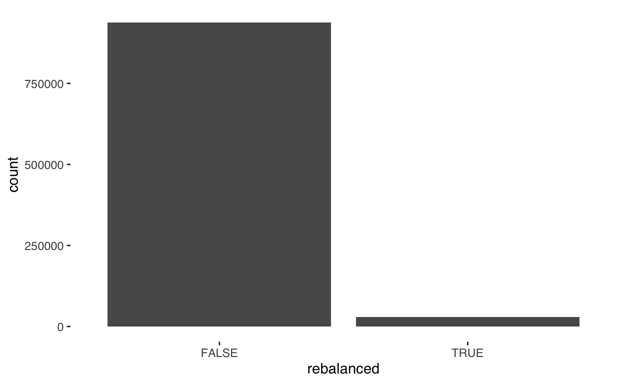
In Python,

ggplot(df_py) + \
geom_bar(
    mapping = aes(x = 'rebalanced'), 
    stat = 'count'
  )

Slide 39

In R, we may code a simple linear regression using the base R function lm like so,

df_r <- df_r %>% mutate(gender_factor = factor(gender) )

model1 <- lm(
  formula = tripduration ~ rebalanced + gender_factor, 
  data = df_r)

summary(model1)

Call:
lm(formula = tripduration ~ rebalanced + gender_factor, data = df_r)

Residuals:
    Min      1Q  Median      3Q     Max 
  -1727    -443    -250      79 2678123 

Coefficients:
               Estimate Std. Error t value Pr(>|t|)    
(Intercept)     1717.67      38.69  44.401   <2e-16 ***
rebalancedTRUE    70.10      42.34   1.656   0.0978 .  
gender_factor1 -1005.53      39.56 -25.418   <2e-16 ***
gender_factor2  -883.02      41.74 -21.153   <2e-16 ***
---
Signif. codes:  0 '***' 0.001 '**' 0.01 '*' 0.05 '.' 0.1 ' ' 1

Residual standard error: 7142 on 967265 degrees of freedom
Multiple R-squared:  0.0006904, Adjusted R-squared:  0.0006873 
F-statistic: 222.7 on 3 and 967265 DF,  p-value: < 2.2e-16

and a generalized linear model using the base R function glm:

model2 <- glm(
  formula = rebalanced ~ tripduration + gender_factor, 
  data = df_r, 
  family = binomial())

summary(model2)

Call:
glm(formula = rebalanced ~ tripduration + gender_factor, family = binomial(), 
    data = df_r)

Coefficients:
                 Estimate Std. Error  z value Pr(>|z|)    
(Intercept)    -3.459e+00  3.148e-02 -109.885  < 2e-16 ***
tripduration    7.722e-07  4.930e-07    1.566   0.1172    
gender_factor1 -5.771e-02  3.224e-02   -1.790   0.0735 .  
gender_factor2  1.610e-01  3.364e-02    4.787 1.69e-06 ***
---
Signif. codes:  0 '***' 0.001 '**' 0.01 '*' 0.05 '.' 0.1 ' ' 1

(Dispersion parameter for binomial family taken to be 1)

    Null deviance: 263044  on 967268  degrees of freedom
Residual deviance: 262799  on 967265  degrees of freedom
AIC: 262807

Number of Fisher Scoring iterations: 6

In Python, we can calculate the same models using the statsmodels library. Here’s the linear model:

import statsmodels.api as sm
import statsmodels.formula.api as smf

df_py = df_py >> mutate(gender_factor = _.gender.astype('category') )
  
model1 = smf.ols(
  formula = 'tripduration ~ rebalanced + gender_factor', 
  data = df_py).fit()

model1.summary()

and here’s the generalized linear model,

model2 = smf.glm(
  formula = 'rebalanced ~ tripduration + gender_factor', 
  data = df_py, 
  family = sm.families.Binomial() ).fit()

model2.summary()