Slide 42 — layering as hierarchy of information
Let’s load libraries for functions we’d like to use,
library(tidyverse) # functions for data transformations, grammar of graphics
library(ggthemes)  # functions for templates of non-data ink
library(ggforce)   # functions for additional geom helper functions
library(ggtext)    # functions to use html/markdown in ggplot fonts
and use a theme to change several aspects of the “non data” ink.
default_theme <- theme_get()
theme_set( theme_classic(base_family = "sans") )
Now let’s simulate some data to graph:
set.seed(15)

n <- 15
d <-
  data.frame(
    x = rnorm(n),
    y = rnorm(n),
    z = rnorm(n),
    a = factor(rpois(n, 1), levels = seq(0, 5)),
    n = seq(n)
  )
Now, we’ll draw the first layer, the main x, y plane:
layer1 <-
  ggplot(d) +

  # coord_equal() +

  scale_x_continuous(
    name = "",
    limits = c(-1.5, 2),
    breaks = seq(-1.5, 1.5, by = 0.5),
    labels = rep("x", 7)
  ) +

  scale_y_continuous(
    name = "",
    limits = c(-1.5, 2),
    breaks = seq(-1.5, 1.5, by = 0.5),
    labels = rep("y", 7)
  ) +

  scale_fill_viridis_d() +

  scale_color_viridis_d() +

  theme(
    legend.position = "",
    # plot.background = element_blank(),
    plot.title = element_text(face = "bold", color = "#444444"),
    plot.subtitle = element_text(color = "#888888"),
    plot.caption = element_text(color = "#888888"),
    axis.text = element_text(color = "#888888"),
    axis.ticks = element_line(color = "#aaaaaa"),
    axis.title = element_text(color = "#888888")
  )

layer1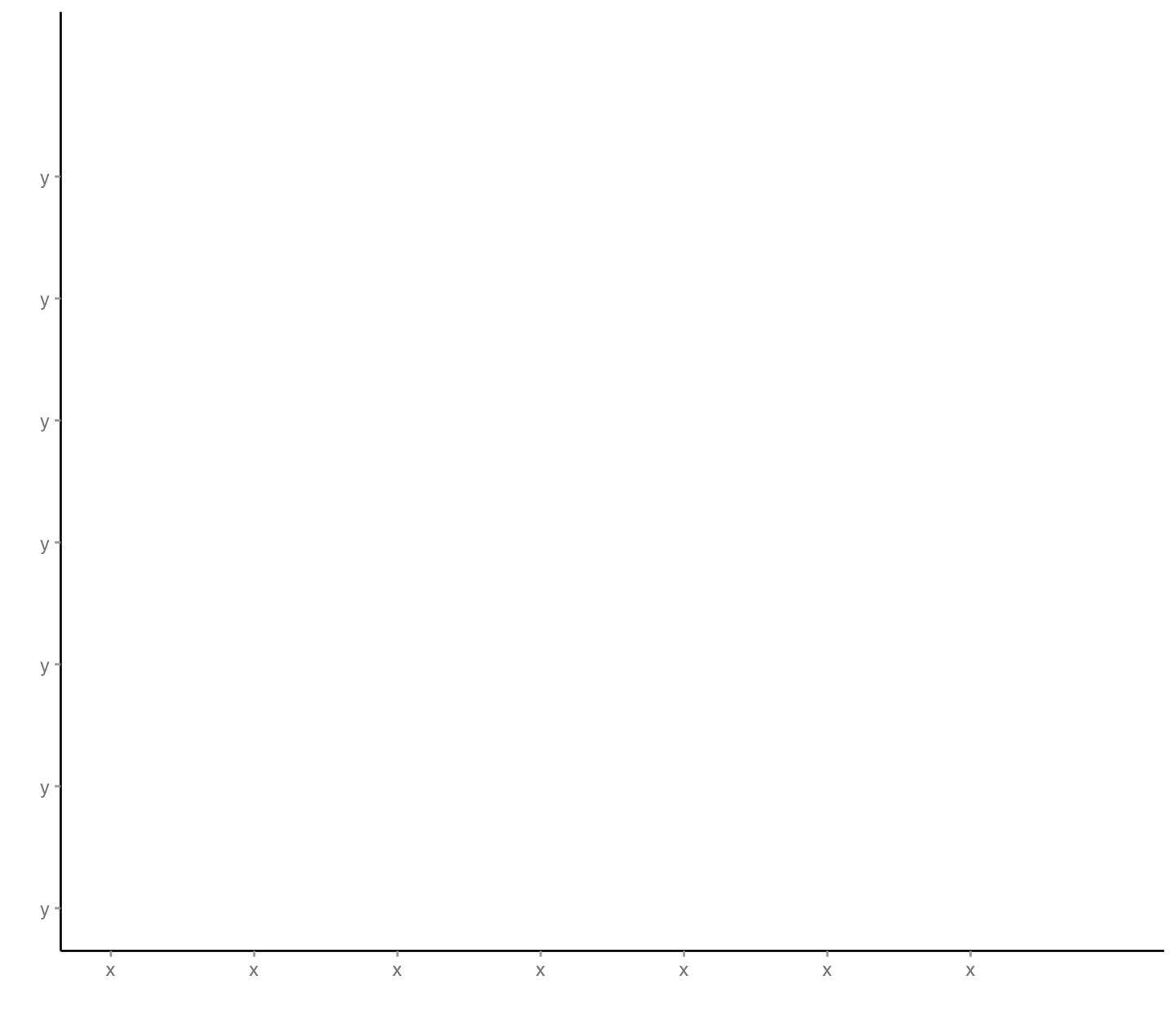
Next, we’ll layer our first two variables onto the x, y coordinates:
layer2 <-

  layer1 +

  geom_point(
    mapping = aes(
      x = x,
      y = y
    )
  )

layer2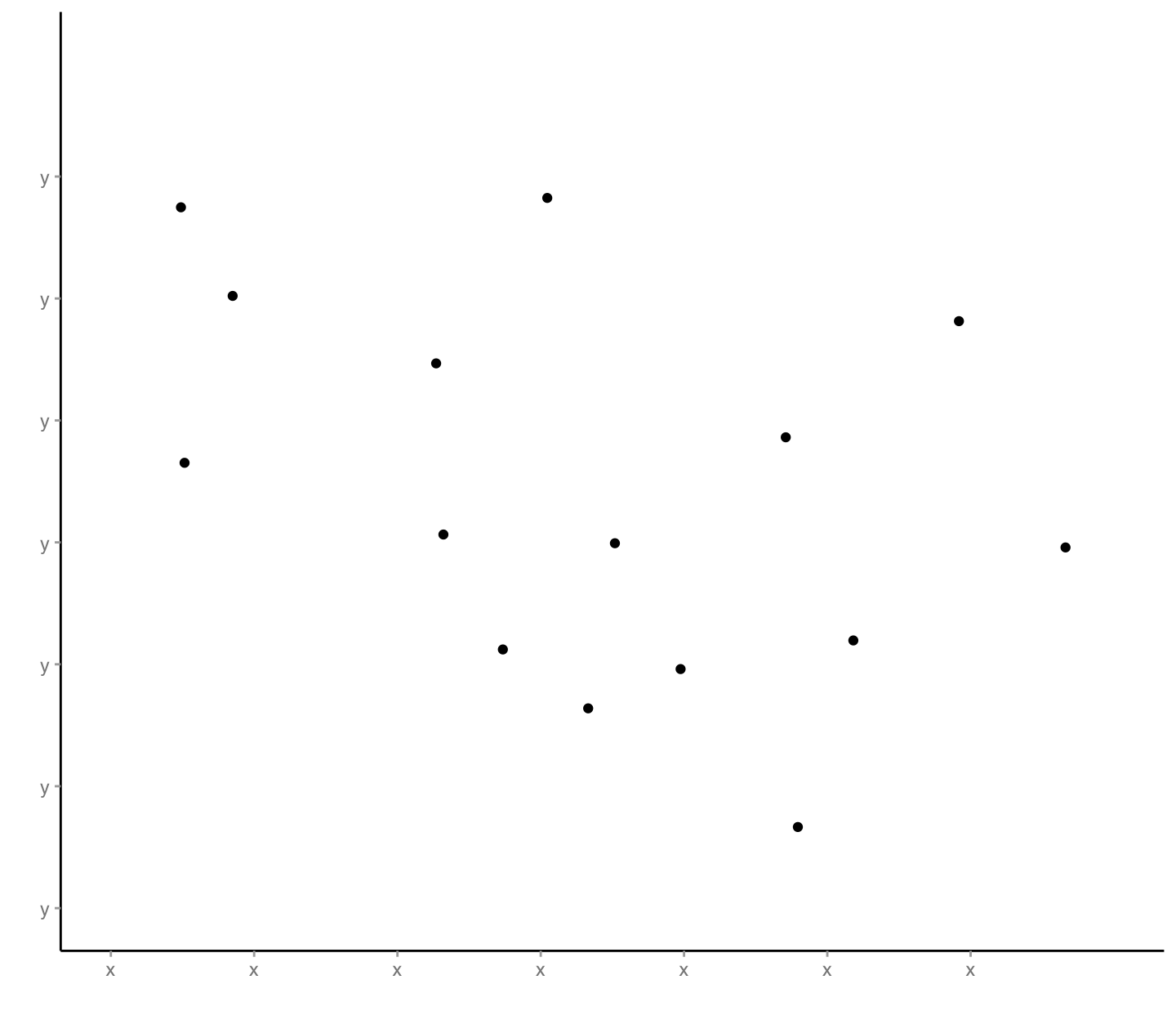
In our third layer, we’ll create custom shapes at the above data-mapped locations where the shapes at those locations in turn depend on data (and so, we get more dimensions to visualize at once):
layer3 <-

  layer1 +

  scale_x_continuous(
    name = "elements positioned by x parameter",
    limits = c(-1.5, 2),
    breaks = seq(-1.5, 1.5, by = 0.5),
    labels = rep("x", 7)
  ) +

  scale_y_continuous(
    name = "elements positioned by y parameter",
    limits = c(-1.5, 2),
    breaks = seq(-1.5, 1.5, by = 0.5),
    labels = rep("y", 7)
  ) +

  geom_rect(
    mapping = aes(
      xmin = x,
      xmax = x + pmax(abs(z) / 4, 0.03),
      ymin = y - 0.03,
      ymax = y + 0.03,
      fill = a
    )
  ) +

  geom_segment(
    mapping = aes(
      x = x,
      xend = x,
      y = y - 0.03,
      yend = y + 0.03
    ),
    color = "#000000",
    lwd = 1
  )

layer3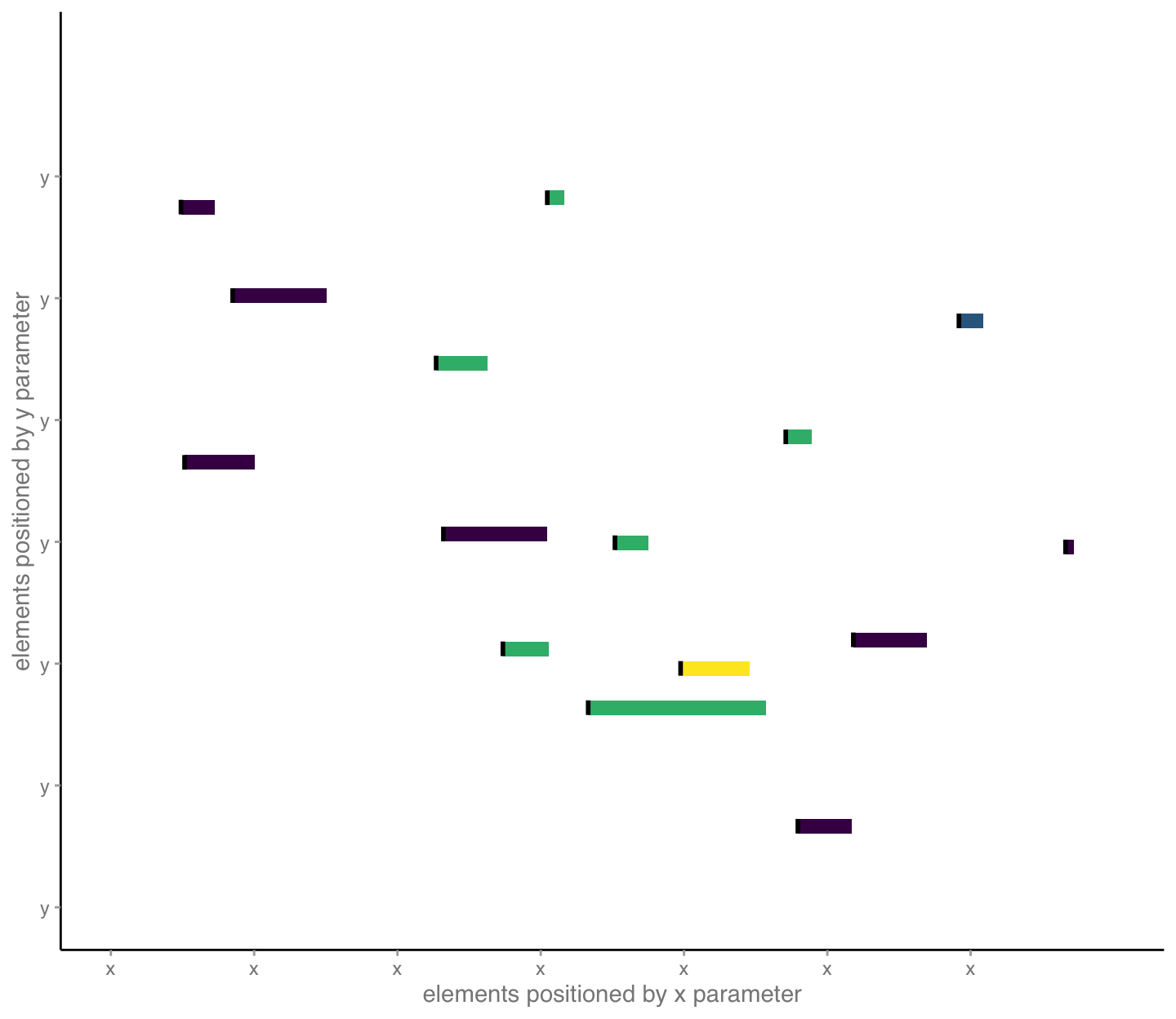
In our forth layer, we begin to include textual details that help our audience understand important aspects of our mappings of data to visual encodings. Here, we label important visual encodings:
layer4 <-

  layer3 +

  geom_text(
    mapping = aes(
      x = x,
      y = y + 0.05,
      label = "name",
      color = a
    ),
    hjust = 0,
    vjust = 0,
    size = 8/.pt,
    fontface = "italic"
  )

layer4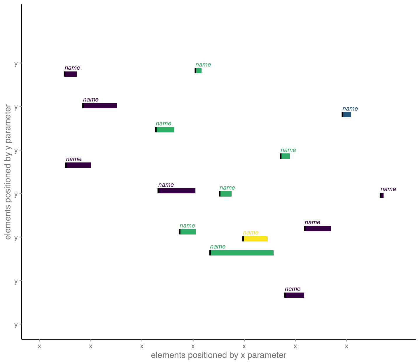
Then, we layer in annotations, tiny paragraphs, that help the audience understand context and insights. Of note, these functions try to automatically place the information and can seem a little finicky, so use a bit of trial and error in re-sizing the figure to work with the placement. Here, a figure size of 7.5 x 6.5 inches for the given font choices seemed pretty good.
layer5 <-

  layer4 +

  geom_mark_rect(
    mapping = aes(
      x = x + 0.06,
      y = y,
      filter = n == 15,
      label = "Explainer",
      description =
        str_c("Use these mini-paragraphs or explainers to say ",
              "something interesting about particular datum. ",
              "Draw your audience in to explore.")
    ),
    label.fontsize = 8,
    con.border = "one",
    con.cap = 0,
    expand = unit(5, "mm"),
    label.colour = "#3e4a89",
    con.colour = "#3e4a89",
    color = "#3e4a89"
  ) +

  geom_mark_rect(
    mapping = aes(
      x = x + 0.09,
      y = y,
      filter = n == 4,
      label = "Explainer",
      description =
        str_c("Use these mini-paragraphs or explainers to say ",
              "something interesting about particular datum. ",
              "Draw your audience in to explore.")
    ),
    label.fontsize = 8,
    con.border = "one",
    con.cap = 0,
    expand = unit(7, "mm"),
    label.colour = "#440154",
    con.colour = "#440154",
    color = "#440154"
  )

layer5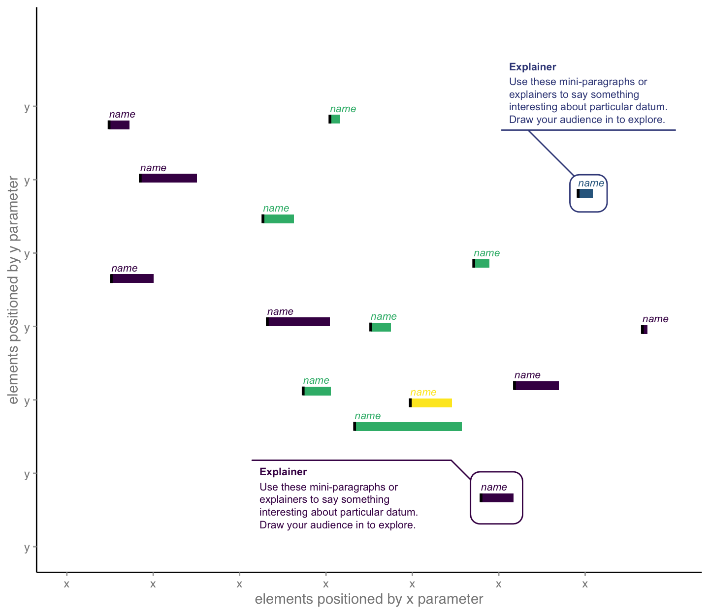
Finally, we add titles, and other surrounding information, to provide messages that provide our audence with added, intelligent insights. We also identify things like data sources and notes to create trust through transparency:
layer6 <-

  layer5 +

  labs(
    title =
      str_c("Use the graphic title to explain your main ",
            "takeaway as it\nrelates to your overall ",
            "narrative, not just what data are shown."),
    subtitle =
      str_c("You can say even more in the subtitle. What ",
            "pattern or comparison did you find\ninteresting? ",
            "By the way, notice the hierarchy of information ",
            "created by font sizes."),
      caption =
      str_c("Source: cite the source of your data ",
            "and explain your analysis.")
  )

layer6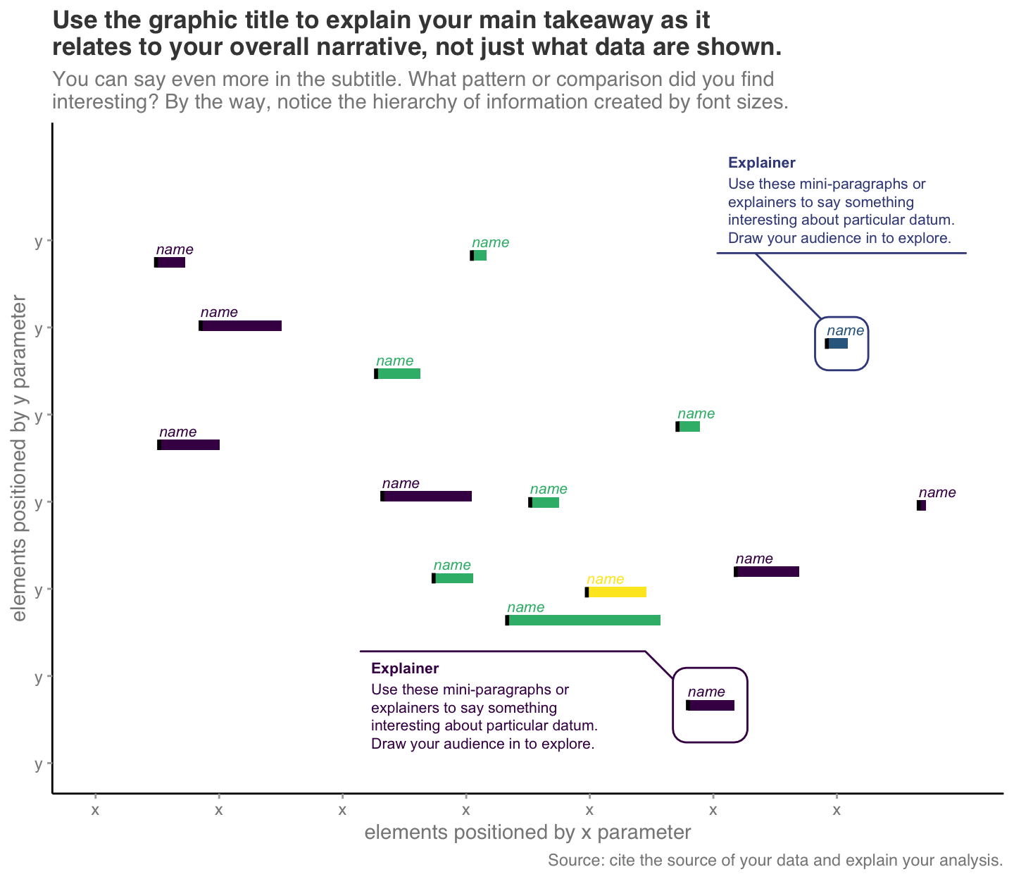
Slide 44 — Data and code for data-ink mappings
I grabbed slightly different years of data (2018-2021) from the US Center for Disease Control and Prevention than used in the NYT graphic (2018).
Here is the website to collect the data.
d_nyt <- read.table( text = '
Cause   Rate    Black   White
Heart   172.6   213.9   166.3
Cancer  150.8   166.4   148.5
COVID19 48.7    69.4    45.9
Accidents   58  60.1    57.4
Cerebrovascular 39.2    54.3    37.2
Diabetes    23.7    41.8    21.3
Homicide    27  26.4    0.4
Lung    26.6    28.8    39.9
Kidney  23  25.3    11.8
Alzheimer   22  28.4    32.3
Hypertension    16.5    18.2    8.7
Septicemia  15.3    16.5    9.5
Flu 13.5    14.9    12.6
Liver   8.8 8.3 13.6
Suicide 7.6 7.5 15.7
',
header = TRUE
)
Here are some grammar of graphics code just to create the data to visual mappings:
d_nyt <-
  d_nyt %>%
  mutate(Difference = Black - White) %>%
  arrange(Difference) %>%
  mutate(
    ymax = cumsum(Rate),
    ymin = lag(ymax, default = 0),
    xcenter = Difference / 2,
    ycenter = (ymin + ymax) / 2
  )

p_nyt1 <-
  ggplot(data = d_nyt) +
  coord_cartesian(
    xlim = c(-30, 55)
  ) +
  geom_rect(
    mapping = aes(
      xmin = 0, xmax = Difference,
      ymin = ymin, ymax = ymax
    ),
    fill = 'lightgray',
    color = 'black'
  ) +
  geom_text(
    mapping = aes(
      x = xcenter,
      y = ycenter,
      label = Cause
    ),
    # can divide by .pt to convert
    # from grid system to font size
    size = 5/.pt
  )

p_nyt1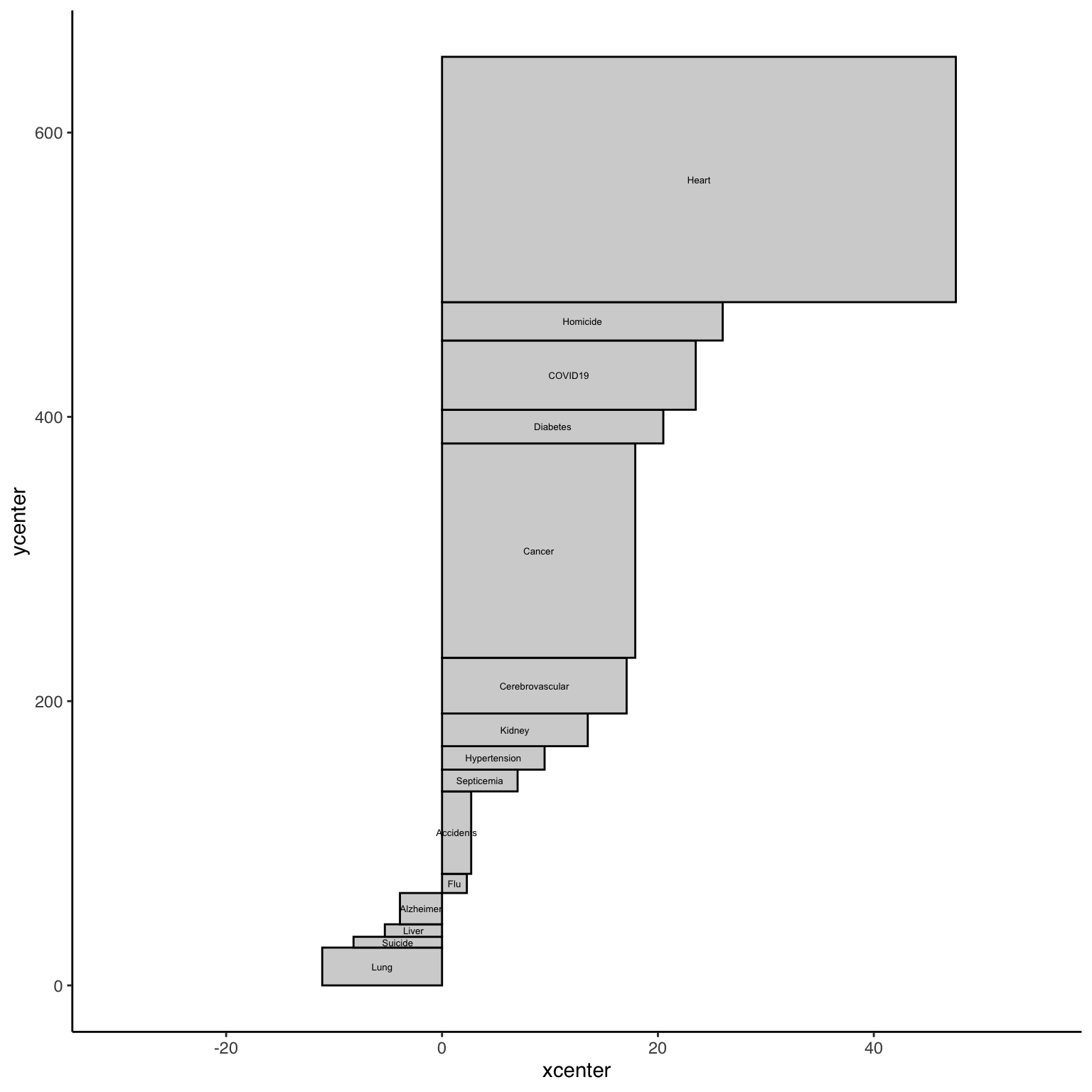
While this alone may be helpful to the research exploring, it would not be sufficient for another audience.
Next, we need to add various text and annotations that would help an audience understand the encodings in a proper context. To do this, consult the functions theme and annotate. Of note, the R package ggthemes includes many default settings for a graph to appear in certain ways. Pro tip: you can see what a specific theme changes by typing its name into the console without including the parenthesis. For example, type theme_tufte without parenthesis, and you’ll see the code changes made using the function theme.
To help match the NYT graphic, I might start with the function theme_classic to remove most things except data-visual mappings, and then add in specific components using the function theme. For example,
p_nyt1 <-
  p_nyt1 +
  theme_void() +
  theme(
    axis.text.x = element_text(),
    panel.grid.major.x = element_line(color = 'lightgray')
    )

p_nyt1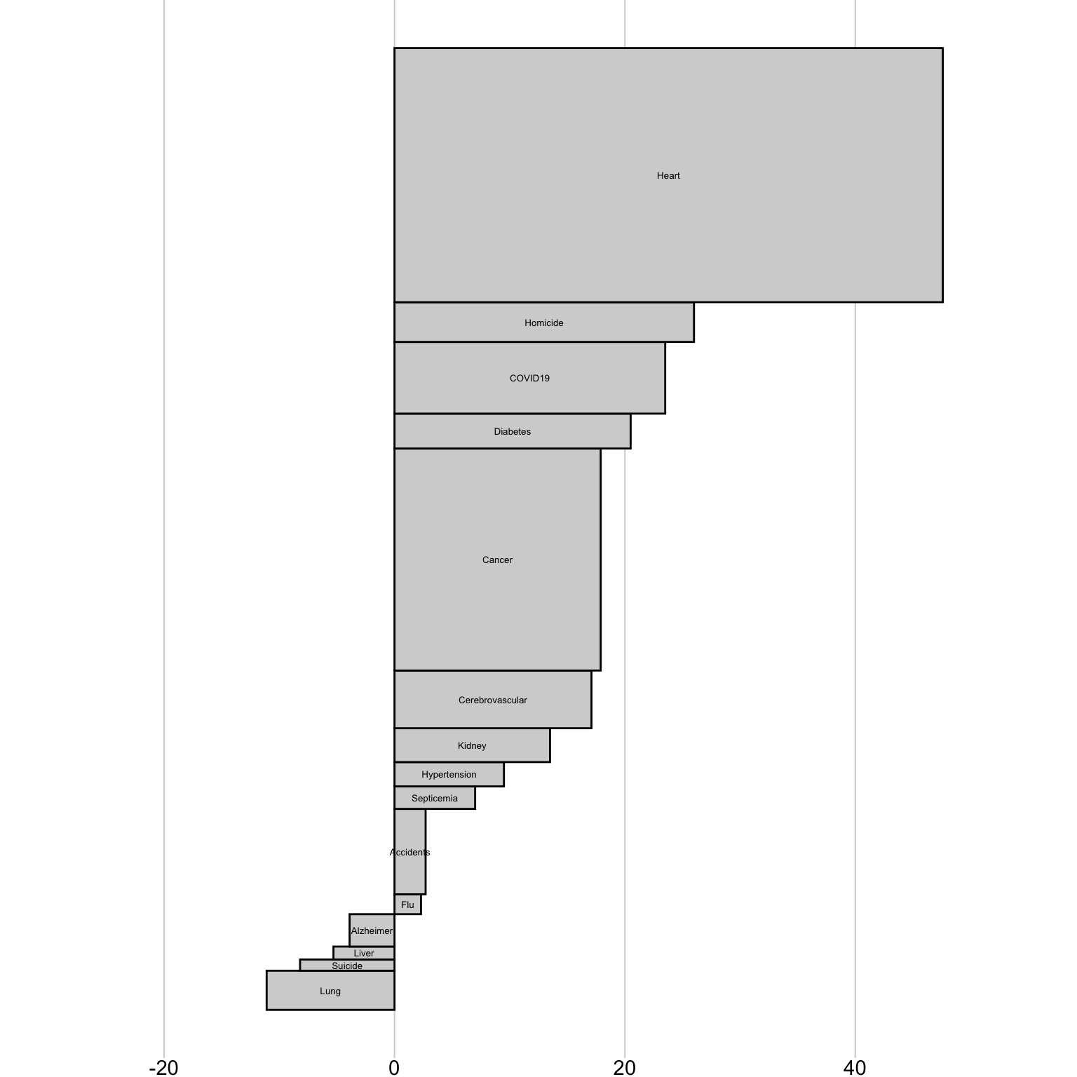
Notice that the NYT graphic moved the x-axis information to the top. Why might that be? We can do that too.
p_nyt1 <-
  p_nyt1 +
  scale_x_continuous(
    position = 'top',
    breaks = seq(-20, 50, by = 10)
  )

p_nyt1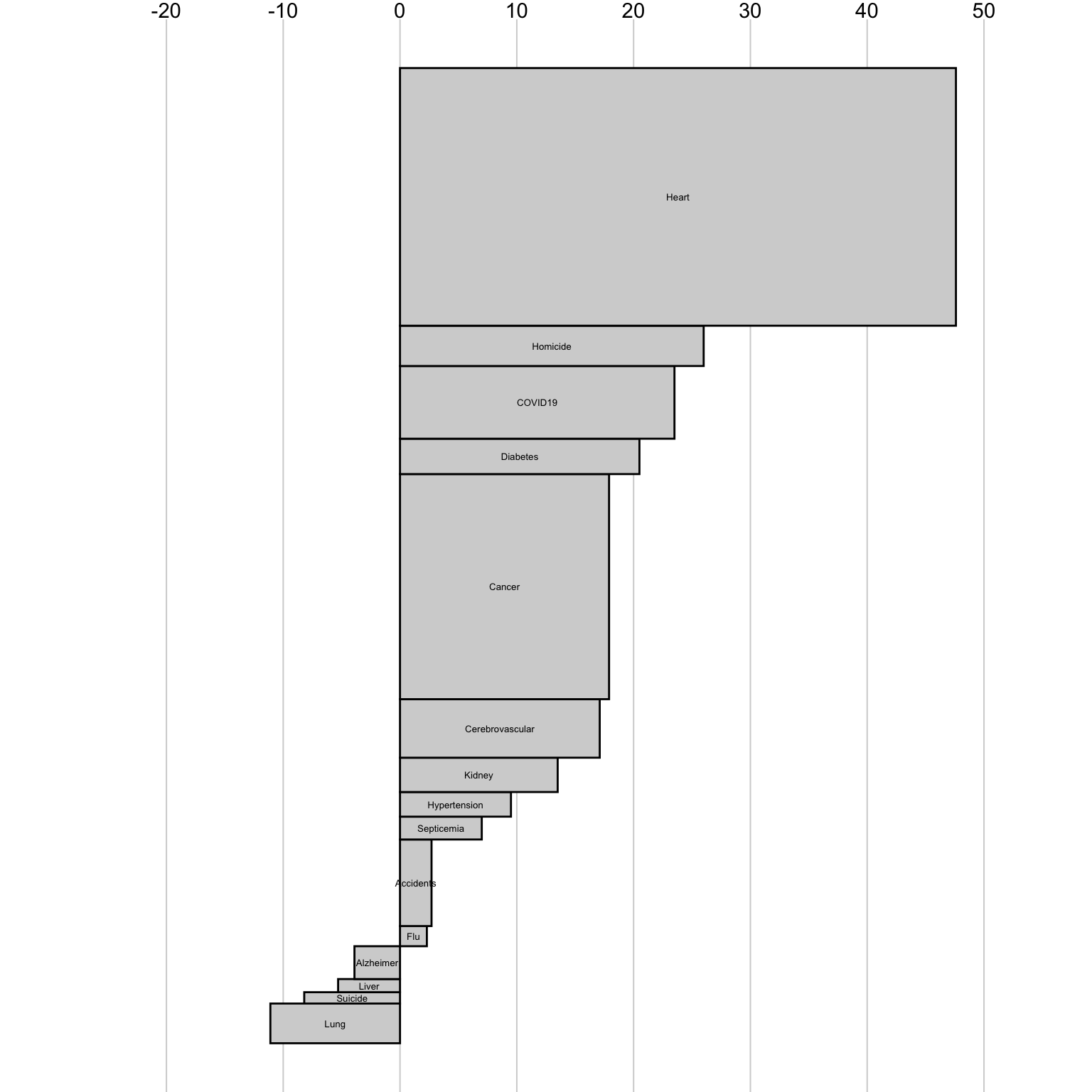
And we can add a title:
p_nyt1 <-
  p_nyt1 +
  labs(
    title = str_c(
      'Gaps between black and white mortality ',
      'rates for the top 15 causes of death')
  ) +
  theme(
    title = element_text(size = 30/.pt)
  )

p_nyt1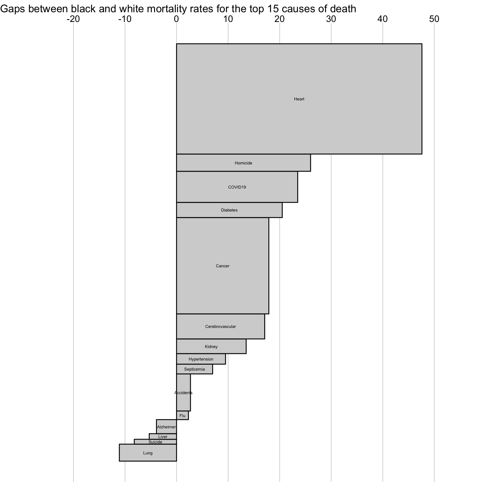
And we can provide general annotations:
p_nyt1 <- p_nyt1 +
  geom_text(
    data = filter(d_nyt, ymax == max(ymax)),
    mapping = aes(x = 2, y = ymax + 20),
    label = 'Higher black death rate ->',
    hjust = 0) +
  geom_text(
    data = filter(d_nyt, ymin == min(ymin)),
    mapping = aes(x = -2, y = ymin - 20),
    label = '<- Higher white death rate',
    hjust = 1)

p_nyt1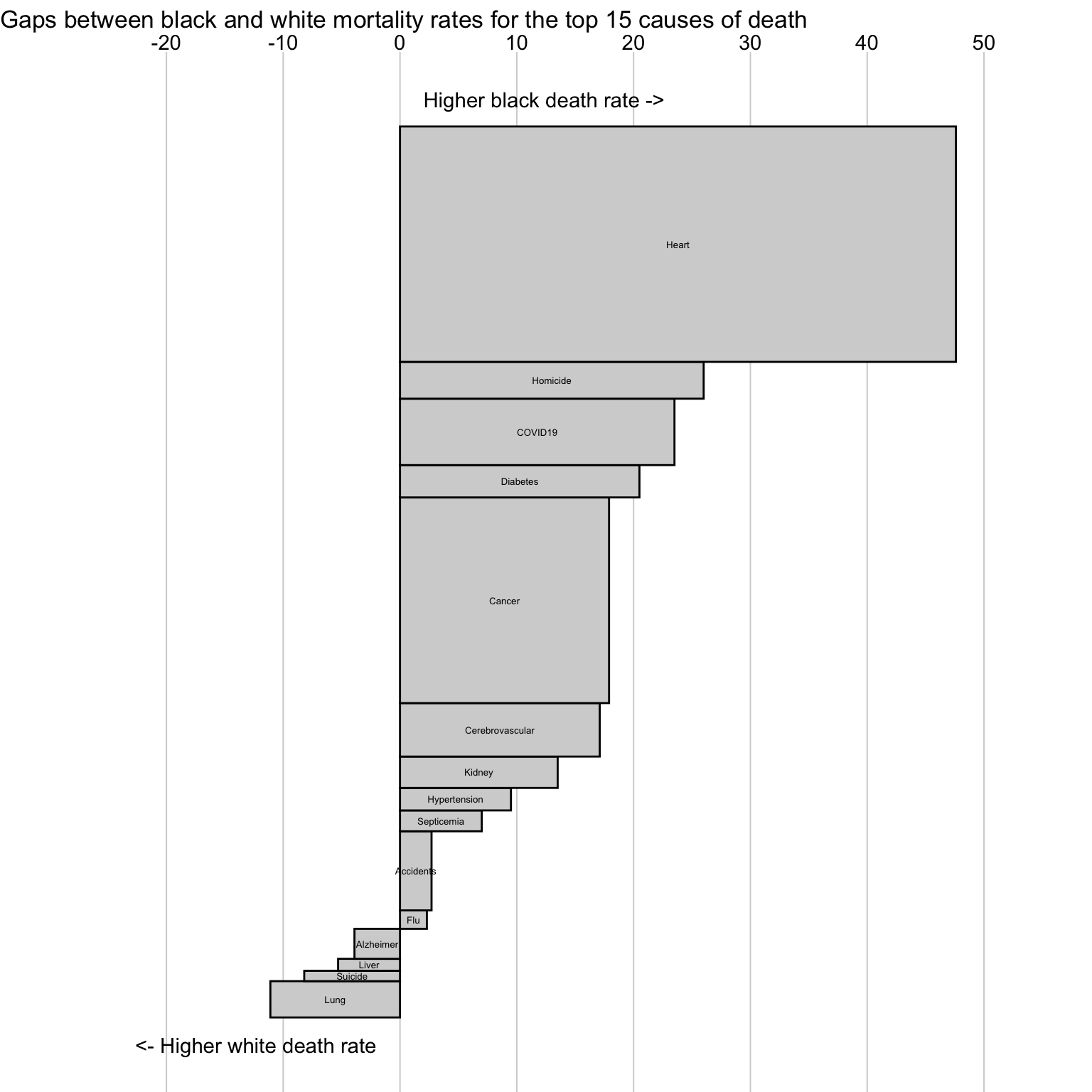
Instead of using the function geom_text in the above, we could have used the function annotate, but the two differ in that the first inherits the data from ggplot while the second does not.
Again, why did the NYT choose to play these two annotations in the locations as published?
Notice that the font sizes look better or worse relative to the graphic depending on the overall size of the graphic. This is one of the most annoying things about this tool for the grammar of graphics. To make it look right, you’ll need to consider the size upfront, and then, adjust the text to your liking.
Also notice that the NYT graphic solved some of the font sizing issue by moving some of the labels outside the rectangles, and providing lines that connect the labels to the rectangles.
As an exercise, try to continue refining this graphic to best mirror that of the NYT graphic.
Slide 52 — BEA data, graphic
We’ll design the following published graphic: Bureau of Economic Analysis. “Gross Domestic Product by Industry: First Quarter 2020.” BEA Statistics. US Department of Commerce, July 6, 2020. https://www.bea.gov/sites/default/files/2020-07/gdpind120-fax.pdf. Here’s the original data that we’ll use to re-design:
d <-
  tribble(
    ~Industry,                             ~Quarter,  ~`Percent change`,
    "Overall GDP",                         "2019:Q4", +0.02,
    "Overall GDP",                         "2020:Q1", -0.05,
    "Finance and insurance",               "2019:Q4", +0.05,
    "Finance and insurance",               "2020:Q1", -0.09,
    "Health care and social assistance",   "2019:Q4", +0.03,
    "Health care and social assistance",   "2020:Q1", -0.078,
    "Arts, entertainment, and recreation", "2019:Q4", -0.01,
    "Arts, entertainment, and recreation", "2020:Q1", -0.347,
    "Accommodation and food services",     "2019:Q4", +0.002,
    "Accommodation and food services",     "2020:Q1", -0.278
  ) %>%
  mutate(
    Industry = factor( Industry, levels = unique(Industry) )
  )
I’ve used a “color picker” to identify each of the colors in the original graphic. Here are the hex codes for them:
bea_colors <- c("#1E4B92", "#97a3b3", "#CA672F", "#E8AC3B", "#DDDDDD")Now, let’s draw the original graphic:
p0 <-

  d %>%

  filter(Industry != "Overall GDP") %>%

  ggplot() +

  scale_fill_manual(
    values = bea_colors
  ) +

  scale_y_continuous(
    breaks = seq(-0.4, 0.1, by = 0.05),
    minor_breaks = NULL,
    limits = c(-0.40, 0.10),
    labels = scales::label_percent(accuracy = 1, suffix = "")
  ) +

  geom_bar(
    mapping = aes(
      x = Quarter,
      y = `Percent change`,
      fill = Industry
    ),
    stat = "identity",
    position = "dodge"
  ) +

  geom_hline(
    mapping = aes(
      yintercept = 0
    ),
    color = "black",
    size = 0.5
  ) +

  labs(
    title = "Real Value Added by Selected Industries",
    caption =
      str_c("U.S. Bureau of Economic Analysis, ",
            "Seasonally adjusted annual rates"),
    x = ""
  ) +

  theme_minimal() +

  theme(
    plot.title = element_text(face = "bold", hjust = 0.5),
    plot.caption = element_text(hjust = 0),
    panel.grid.major.x = element_blank(),
    panel.grid.major.y = element_line(size = 0.8),
    axis.text = element_text(face = "bold", size = 36/.pt),
    axis.title = element_text(face = "bold")
  )

p0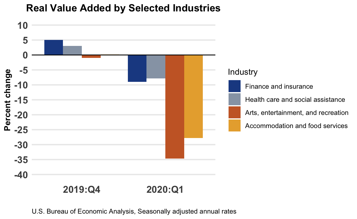
Slide 53 — redesign 1
Let’s try a different approach to both mapping the data and providing better textual details:
p1 <-

 d %>%

 ggplot() +

 theme_tufte() +

 scale_x_discrete(position = "top") +

 scale_y_continuous(
   breaks = seq(-0.4, 0.1, by = 0.1),
   minor_breaks = seq(-0.4, 0.1, by = 0.05),
   limits = c(-0.35, 0.07),
   labels = scales::label_percent(accuracy = 1, suffix = "")
 ) +

 scale_fill_manual(
   values = c("gold", "skyblue", "lightgray")
 ) +

 theme(
   plot.title = element_text(face = "bold", size = 48/.pt),
   plot.caption = element_text(hjust = 0),
   axis.title = element_blank(),
   axis.text.y = element_text(face = "bold", size = 30/.pt),
   axis.ticks = element_blank(),
   axis.text.x = element_text(face = "bold", size = 30/.pt),
   legend.position = "top",
   panel.grid.major.y = element_line(color = "#bbbbbb", linetype = "dotted"),
   panel.grid.minor.y = element_line(color = "#bbbbbb", linetype = "dotted")
 ) +

 geom_bar(
   mapping = aes(
     x = Industry,
     y = `Percent change`,
     fill = Quarter
   ),
   stat = "identity",
   position = position_dodge(),
   width = 0.7
 ) +

 geom_bar(
   data = filter(d, Industry == "Overall GDP"),
   mapping = aes(
     x = Industry,
     y = `Percent change`,
     group = Quarter
   ),
   stat = "identity",
   position = position_dodge(),
   width = 0.8,
   fill = "#dddddd"
 ) +

 geom_text(
   data = filter(d, Industry == "Overall GDP"),
   mapping = aes(
     x = Industry,
     y = sign(`Percent change`) * 0.01,
     label = Quarter,
     group = Quarter
   ),
   stat = "identity",
   position = position_dodge(width = 0.8),
   hjust = 0.5
 ) +

 geom_vline(xintercept = 1.5, color = "#dddddd") +

 geom_hline(yintercept = 0) +

 labs(
   title =
     str_c("As the pandemic set hold, most industries ",
           "shrank in real value\nadded to GDP, food ",
           "services and recreation more so than others."),
   subtitle = "(Percent change from previous quarter)",
   caption =
     str_c("Source: U.S. Bureau of Economic Analysis, ",
           "Seasonally adjusted annual rates")
 )

# note that we can set the width and height in the r markdown code chunk
# options, we I did for those in slide 44, or we can do something like
# this too:

ggsave("redesign01.svg", plot = p1, width = 15, height = 5)
knitr::include_graphics("redesign01.svg")
Slide 54 — redesign 2
Let’s try a second design.
p2 <-

 d %>%

 ggplot() +

 theme_tufte() +

 theme(
   plot.title = element_text(face = "bold", size = 48/.pt),
   plot.caption = element_text(hjust = 0),
   axis.title = element_blank(),
   axis.text.y = element_blank(),
   axis.ticks = element_blank(),
   axis.text.x = element_text(face = "bold", size = 36/.pt),
   legend.position = "top"
 ) +

 scale_x_continuous(
   breaks = seq(-0.4, 0.1, by = 0.05),
   minor_breaks = NULL,
   limits = c(-0.40, 0.20),
   labels = scales::label_percent(accuracy = 1, suffix = "")
 ) +

 scale_color_manual(
   values = c("gold", "skyblue")
 ) +

 geom_vline(
   xintercept = 0,
   color = "lightgray"
 ) +

 geom_line(
   mapping = aes(
     x = `Percent change` + if_else(Quarter == "2020:Q1", +0.006, -0.006),
     y = Industry,
     group = Industry
   ),
   size = 1,
   arrow = arrow(ends = "first", type = "closed", length = unit(0.2, "cm"))
 ) +

 geom_point(
   mapping = aes(
     x = `Percent change`,
     y = Industry,
     color = Quarter,
   ),
   size = 4
 ) +

 geom_label(
   data = filter(d, Quarter == "2019:Q4"),
   mapping = aes(
     x = `Percent change`,
     y = Industry,
     label = as.character(Industry),
   ),
   hjust = 0,
   nudge_x = 0.005,
   fontface = "bold",
   label.size = NA
 ) +

 labs(
      title =
        str_c("As the pandemic set hold, most industries ",
              "shrank in real value\nadded to GDP, food ",
              "services and recreation more so than others."),
      subtitle = "(Percent change from previous quarter)",
      caption =
        str_c("Source: U.S. Bureau of Economic Analysis, ",
              "Seasonally adjusted annual rates")
 )

ggsave("redesign02.svg", plot = p2, width = 15, height = 5)
knitr::include_graphics("redesign02.svg")
Slide 55 — redesign 3
And a third redesign. Try to think closely about what we are making comparisons between and how.
p3 <-
 d %>%

 ggplot() +

 theme_void() +

 theme(
   plot.title = element_markdown(face = "bold", size = 48/.pt),
   plot.caption = element_text(hjust = 0, size = 30/.pt),
   axis.text.x = element_text(face = "bold", size = 36/.pt),
   legend.position = ""
 ) +

 scale_color_manual(
   values = c("#000000", "#CA672F", "#E8AC3B", "#1E4B92", "#97a3b3")
 ) +

 scale_x_discrete(
   expand = expansion(add = c(0.8, 0.7))
 ) +

 scale_y_continuous(
   limits = c(-0.35, 0.07),
   labels = scales::label_percent(accuracy = 1, suffix = "")
 ) +

 geom_hline(
   yintercept = 0,
   color = "#888888",
   linetype = "dotted"
 ) +

 annotate(
   "text",
   x = "2020:Q1",
   y = +0.01,
   label = "↑ expanding from previous period",
   fontface = "bold",
   hjust = 0
 ) +

 annotate(
   "text",
   x = "2020:Q1",
   y = -0.01,
   label = "↓ shrinking",
   fontface = "bold",
   hjust = 0
 ) +

 geom_line(
   mapping = aes(
     x = Quarter,
     y = `Percent change`,
     group = Industry,
     color = Industry
   ),
   size = 1,
   arrow = arrow(ends = "last", type = "closed", length = unit(0.2, "cm"))
 ) +

 geom_label(
   data = filter(d, Quarter == "2019:Q4"),
   mapping = aes(
     x = Quarter,
     y = `Percent change`,
     label = str_c(as.character(Industry), " ",
                   str_c(format(`Percent change` * 100, 1), "%")),
     color = Industry
   ),
   hjust = 1,
   nudge_x = 0.005,
   fontface = "bold",
   label.size = NA
 ) +

 geom_label(
   data = filter(d, Quarter == "2020:Q1"),
   mapping = aes(
     x = Quarter,
     y = `Percent change`,
     label = str_c(format(`Percent change` * 100, 1), "%"),
     color = Industry
   ),
   hjust = 0,
   nudge_x = 0.005,
   fontface = "bold",
   label.size = NA
 ) +

 labs(
   title =
     str_c("As the pandemic set hold, most industries ",
           "shrank in real value<br>added to GDP, ",
           "<span style='color:#97a3b3;'>food ",
           "services</span> and <span style='color:#1E4B92;'>",
           "recreation</span> worse than others."),
   subtitle = "(Percent change from previous quarter)",
   caption =
     str_c("Source: U.S. Bureau of Economic Analysis, ",
           "Seasonally adjusted annual rates")
 )

ggsave("redesign03.svg", plot = p3, width = 15, height = 15)
knitr::include_graphics("redesign03.svg")
What other redesigns did you consider?