7. Storytelling with data

Example code used in class discussion.

Slide 13

Load libraries to use data transformation and graphing functions.

library(tidyverse)  # usual data transformations and grammar of graphics
library(ggthemes)   # for setting defaults on non-data ink
library(tidycensus) # for gathering US census county ids and populations
theme_set( theme_void() + theme(legend.position = "") )

Pull census data, including county ids and population thereof.

CENSUS_API_KEY <- Sys.getenv("CENSUS_API_KEY")

county_pop <- get_estimates(
  geography = "county",
  product = "population",
  year = 2019,
  key = CENSUS_API_KEY)

Slides 13-20 - simulate per-county cancer rates

set.seed(1)

data <- 
  county_pop %>%
  pivot_wider(
    names_from = "variable", 
    values_from = "value") %>%
  left_join(county_laea) %>%
  rowwise() %>%
  mutate(
    rate_cases = rbinom(n = 1, size = POP, prob = 0.01) / POP * 1000
  )

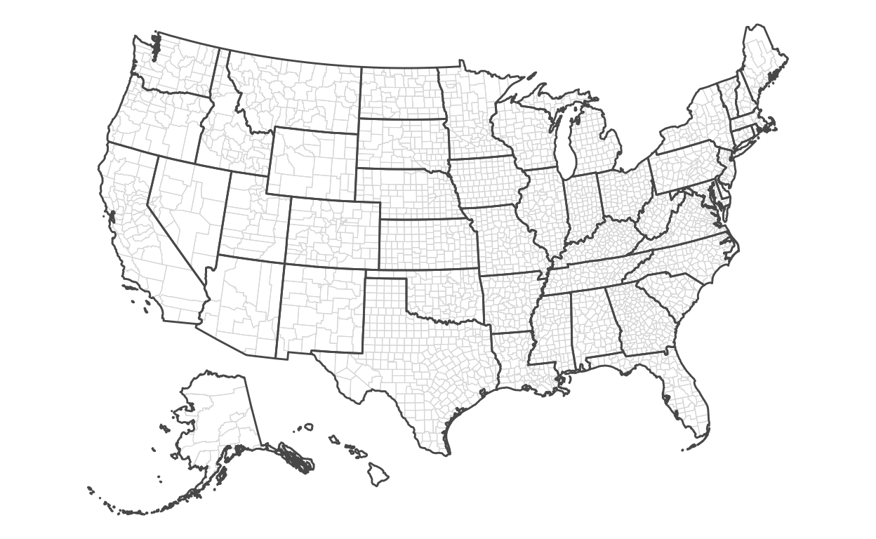
Slide 13 - map encoding county areas

ggplot() + 
  theme_void() + 
  theme(legend.position = "") +
  geom_sf(
    data = data, 
    mapping = aes(
      geometry = geometry),
    lwd = 0.2,
    color = '#dddddd',
    fill = NA
  ) +
  geom_sf(
    data = state_laea,
    fill = NA
  )

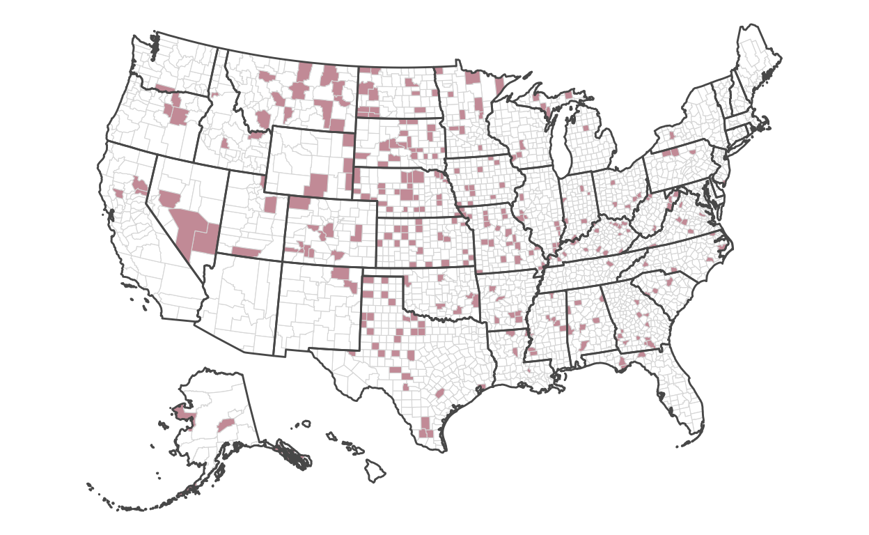
Slide 14 - map encoding counties with hightest rates

ggplot() + 
  geom_sf(
    data = data, 
    mapping = aes(
      geometry = geometry,
      fill = rate_cases > quantile(rate_cases, probs = 0.9)
    ),
    lwd = 0.2,
    color = '#dddddd'
  ) +
  geom_sf(
    data = state_laea,
    fill = NA
  ) +
  scale_fill_manual(
    values = c("#ffffff", "#CD9DA7")
  )

Slide 15 - map encoding counties with lowest rates

ggplot() +
  geom_sf(
    data = data, 
    mapping = aes(
      geometry = geometry,
      fill = rate_cases < quantile(rate_cases, probs = 0.1)
    ),
    lwd = 0.2,
    color = '#dddddd'
  ) +
  geom_sf(
    data = state_laea,
    fill = NA
  ) +
  scale_fill_manual(
    values = c("#ffffff", "#6695BC")
  )

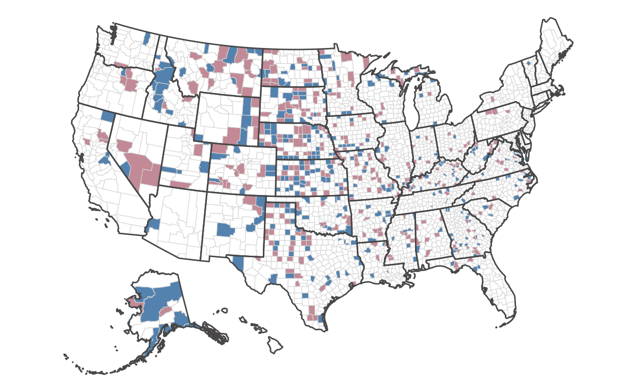
Slide 16 - map encoding lowest and hightest rates

ggplot() + 
  scale_fill_identity() +
  geom_sf(
    data = data, 
    mapping = aes(
      geometry = geometry,
      fill = case_when(
        rate_cases > quantile(rate_cases, probs = 0.9) ~ "#CD9DA7",
        rate_cases < quantile(rate_cases, probs = 0.1) ~ "#6695BC",
        TRUE ~ "#ffffff")
      ),
    lwd = 0.2,
    color = '#dddddd'
  ) +
  geom_sf(
    data = state_laea,
    fill = NA
  )

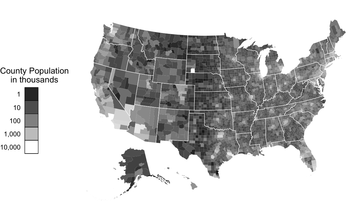
Slide 18 - map encoding county populations

ggplot() +
  theme_void() +
  geom_sf(
    data = data, 
    mapping = aes(
      geometry = geometry,
      fill = POP ),
    lwd = 0.2,
    color = NA) +
  geom_sf(
    data = state_laea,
    fill = NA,
    color = '#ffffff',
    lwd = 0.2
  ) +
  scale_fill_gradient(
    low = '#000000',
    high = '#ffffff',
    name = 'County Population\nin thousands', 
    trans = 'log10',
    breaks = c(0, 1e3, 1e4, 1e5, 1e6, 1e7),
    labels = c(0, "1", "10", "100", "1,000", "10,000")
  ) +
  theme(
    legend.position = 'left', 
    legend.text.align = 1,
    legend.title = element_text(hjust = 0),
    legend.key = element_rect(color = '#000000')
  ) +
  guides(
    fill = guide_legend(
      title.position = "top", 
      title.hjust = 0.5,
      label.position = "left"
    )
  ) 

Slide 20 - graph encoding rates ~ population

ggplot(data) +
  theme_tufte(base_family = 'sans') +
  geom_point(
    mapping = aes(
      x = POP,
      y = rate_cases,
      color = case_when(
        rate_cases > quantile(rate_cases, probs = 0.9) ~ '#CD9DA7',
        rate_cases < quantile(rate_cases, probs = 0.1) ~ '#6695BC',
        TRUE ~ '#000000'
      )
    ),
    size = 1.5,
    alpha = 0.6,
    shape = 21
  ) +
  geom_hline(
    mapping = aes(
      yintercept = quantile(rate_cases, probs = 0.9)
    ),
    linetype = 'dotted',
  ) +
  annotate(
    'text',
    x = 1e6,
    y = quantile(data$rate_cases, probs = 0.9) + 0.2,
    label = "↑ 90th Percentile",
    hjust = 0,
    vjust = 0,
    color = '#CD9DA7'
  ) +
  geom_hline(
    mapping = aes(
      yintercept = quantile(rate_cases, probs = 0.1)
    ),
    linetype = 'dotted'
  ) +
  annotate(
    'text',
    x = 1e6,
    y = quantile(data$rate_cases, probs = 0.1) - 0.2,
    label = "↓ 10th Percentile",
    hjust = 0,
    vjust = 1,
    color = '#6695BC'
  ) +
  scale_x_log10(
    breaks = c(0, 1e3, 1e4, 1e5, 1e6, 1e7),
    labels = c(0, "1", "10", "100", "1,000", "10,000")) +
  scale_color_identity() +
  theme(legend.position = '') +
  labs( 
    x = "County populations in thousands",
    y = "Age-adjusted rates of cancer per 1,000 people"
  )