10. Storytelling with data

Example code used in class discussion.

libraries

library(tidyverse)
library(ggiraph)
library(patchwork)

Slide 21

load data

fields <- readRDS("data/outfields.rds")
fields <- 
  fields %>% 
  mutate(
    is_infield = ifelse(id > 30, TRUE, FALSE),
    ysh = -ysh
  )

fences <- readRDS("data/fences.rds")
fences <- fences %>% mutate(ysh = -ysh)

static grammar of graphics plot

gg_boundaries <-
  ggplot() + 
  theme_void() + 
  coord_equal() +
  geom_path(
    data = subset(
      fields, 
      is_infield == FALSE),
    mapping = aes(
      x = xsh,
      y = ysh,
      group = id),
    color = '#000000',
    alpha = 0.5) +

  geom_polygon(
    data = subset(
      fields, 
      is_infield == TRUE),
    mapping = aes(
      x = xsh,
      y = ysh,
      group = id),
    fill = '#FAD9B4',
    color = '#FAD9B4') 

gg_boundaries

Slide 22

library(ggiraph)

gg_boundaries <- 
  ggplot() + 
  theme_void() + 
  coord_equal() +
  geom_path_interactive(
    data = subset(
      fields, 
      is_infield == FALSE),
    mapping = aes(
      x = xsh,
      y = ysh,
      group = id,
      tooltip = id, 
      data_id = id
      ),
    color = '#000000',
    alpha = 0.5) +
  
  geom_polygon(
    data = subset(
      fields, 
      is_infield == TRUE),
    mapping = aes(
      x = xsh,
      y = ysh,
      group = id),
    fill = '#FAD9B4',
    color = '#FAD9B4')

girafe(
  code = print(gg_boundaries),
  options = list(
    opts_hover(
      css = 'stroke-width:3;'),
    opts_hover_inv(
      css = 'stroke-opacity:0.1;')
    )
  )

Slide 24

gg_fences <- 
    ggplot() + 
    theme_void() +
    theme( axis.text.x = element_text() ) +
    coord_equal() +
    scale_x_continuous(
      breaks = c(100, 300, 500), 
      labels = c("Left Field", 
                 "Center Field", 
                 "Right Field")) +
    geom_path_interactive(
      data = fences,
      mapping = aes(
        x = xsh,
        y = -ysh,
        group = id,
        tooltip = id, 
        data_id = id),
      color = 'black',
      alpha = 0.5)

girafe(
  code = print(gg_boundaries / gg_fences),
  options = list(
    opts_hover(
      css = 'stroke-width:3;'),
    opts_hover_inv(
      css = 'stroke-opacity:0.1;')
    )
  )

Slide 26

library(plotly)
library(crosstalk)
library(DT)

m <- highlight_key(mpg)

p <- ggplot(
  data = m, 
  mapping = aes(
   x = displ, 
   y = hwy)) + 
  geom_point()

gg <- highlight(
  p = ggplotly(p), 
  on = "plotly_selected")

bscols(gg, datatable(m))

Slide 28

library(r2d3)
bars <- c(10, 20, 30)

svg.selectAll('rect')
  .data(data)
  .enter()
    .append('rect')
      .attr('width', function(d) { return d * 10; })
      .attr('height', '20px')
      .attr('y', function(d, i) { return i * 22; })
      .attr('fill', 'orange');

Slide 31

This is sample content placed in the area defined by our title class.

This is sample content placed in the area defined by our large-left class.

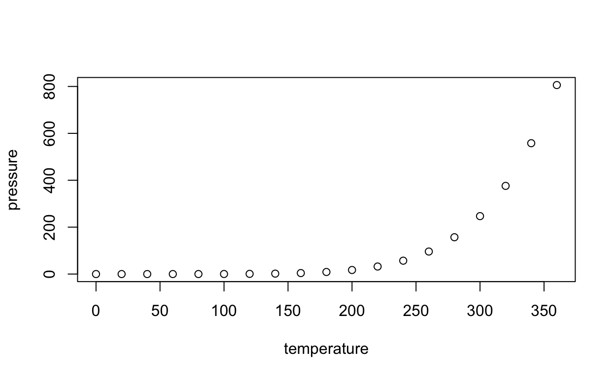
plot(pressure)

This is sample content placed in the area defined by our medium-middle class.

plot(pressure)

This is sample content placed in the area defined by our medium-right class.

plot(pressure)

This is sample content placed in the area defined by our bottom-full class.

plot(pressure)

This is sample content placed in the area defined by our bottom-middle class.

plot(pressure)

This is sample content placed in the area defined by our bottom-right class.

plot(pressure)